Optimization via Infill Criteria using Surrogates
When dealing with a non linear problem (NLP), such as in (3), typically it is resorted to classical solvers (e.g. SQP, trust-region-dogleg, genetic algorithms, simulated annealing, etc.) to obtain its solution, depending on the nature of the NLP (e.g. presence of discontinuities, whether or not the function is differentiable, etc.).
There is a entire field of study dedicated to find these NLP solutions with Kriging surrogates. In the works of [20][30][11][1], there are entire discussions and frameworks on how to solve non linear problems and comparisons of several metrics involved in the optimization process with metamodels.
The premise of performing a optimization using surrogates is that the model to be optimized is too time consuming or computationally expensive to be solved with classical solvers. To circumvent this, the following steps are proposed:
Build an approximation model with Kriging surrogates using a limited number of initial samples. This approximation is a “generalist” enough representation of the real model;
Perform an optimization of the approximation model using classical NLP solvers and an infill criteria. The surrogate model reduces the “search area” needed by the solver;
Compare the surrogate optimum found in step 2 with the result from original model. In other words: feed the results from the Kriging metamodel optimum into the original model and see if they are close enough;
If the optimum from the metamodel is close enough (based on a chosen metric) to the original model, then this may be the true optimum. Otherwise, update the Kriging model by introducing the value found and return to step 2;
This process is basically “filling holes” (hence the name infill) in our Kriging metamodel until original model optimum is found. To illustrate this in the simplest way, we are going to use the same function (24).
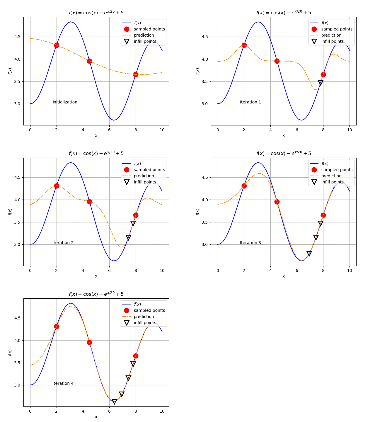
Assuming that we only have three initial points sampled from this model function, we build our Kriging model. As can be seen in Fig. 126.
Fig. 126 Initial plot of the example function. The solid blue line represents the function behavior. The orange dashed line is the Kriging metamodel of the three sampled points (red circles) available.
When applying an optimization solver on the Kriging model, we get a new optimal value for \(x\) near 7.8 (3.47 for \(f(x)\)) in the sample and rebuild the Kriging metamodel. The result is shown Fig. 127. We keep repeating this procedure until we get the result in Fig. 128.
Fig. 127 The Kriging model after one update.
Fig. 128 The Kriging model after four updates. Notice how the Kriging model adjusts to the true function near the optimal point.
This is the entire process animated in Fig. 129:

Fig. 129 The main steps of the infill criteria procedure as an example.
This example is a trivial one because the problem involves a single input variable and infill criteria is the own Kriging prediction of the model. As discussed in [20], this criteria has its pitfalls if used without other precautions.
[6] presented an algorithm, based on the “method 2” in the work of [20], referred as a gradient matching technique where the gradient of the surrogate is forced to match with the true function gradient, this is done through trust-region approach to ensure local convergence which was proven in the work of [1].
Important
The basic idea of this approach is:
Minimize the NLP problem metamodel.
Consult the original function at the minimum found in the metamodel.
Update the sample matrix used to build the surrogate.
Repeat this until a convergence criteria is met.
The flowchart depicting the whole procedure is defined in Fig. 130. For detailed explanation of each step of the proposed algorithm, one must refer to [6] and [3].