Surrogate modeling - Kriging

Metamodels are a way to represent the world in simpler terms. Think of them as a photograph, they do not capture the moment as whole but can represent it good enough. In this analogy, the moment is a complex process that it is too cumbersome to explain it completely in mathematical terms, and metamodels, as photographs, may serve the purpose of capturing the core trends of this process without being too unwieldy and not losing too much information.

There is a family of metamodeling methodologies, ranging from a simple linear regression to complex neural networks. However, the surrogate methodology currently implemented in Metacontrol is the Kriging.

The simplest form to represent a real world process (\(y\)) through a metamodel (\(\hat{y}\)) and its error (\(\varepsilon\)) is done through (17).

(17)\[y(x) = \hat{y}(x) + \varepsilon\]

The error (\(\varepsilon\)) is associated with the unmodeled effects of the inputs (\(x\)) and random noise (i.e. it cannot be explained in detail but cannot be ignored as well.). When using the Kriging methodology as metamodel, this error is assumed to be a probabilistic function of \(x\), or in other words, this error is assumed to be not independent and identically distributed. The specific probabilistic function is represented by a Gaussian distribution with mean (\(\mu\)) zero and variance \(\sigma^2\).

As from [26], a Kriging metamodel \(\hat{y}(x)\), of a rigorous model \(y(x)\) of \(q\) dimensions, is comprised of two parts: a polynomial regression (\(\mathcal{F}\)) and departure function (\(z\)) of stochastic nature:

\[\hat{y}_{l}(x)=\mathcal{F}\left(\beta_{:, l}, x\right)+z_{l}(x), \quad l=1, \ldots, q\]

The regression model, considered as a linear combination of (\(t\)) functions (\(f_{j}: \mathbb{R}^{n} \rightarrow \mathbb{R}\)), as defined in (18).

(18)\[ \mathcal{F}\left(\beta_{:, l}, x\right) \equiv f(x)^{T} \beta_{:, l}\]

The most common choices for \(f(x)\) are polynomials with orders ranging from zero (constant) to two (quadratic). It is assumed that \(z\) has mean zero, and the covariance between to given points, arbitrarily named \(w\) and \(x\) for instance, is defined by (19):

(19)\[\operatorname{Cov}\left[z_{l}(w), z_{l}(x)\right]=\sigma_{l}^{2} \mathcal{R}\left(\theta_{l}, w, x\right), \quad l=1, \ldots, q\]

With \(\sigma_{l}^{2}\) being the process variance for the lth response component, and \(\mathcal{R}(\theta, w, x)\) defined as the correlation model. In Metacontrol, the correlation model used is described by (20).

(20)\[\mathcal{R}\left(\theta_{l}, w, x\right)=\exp \left(-\sum_{i=1}^{m} \theta_{l}\left(w-x_{i}\right)^{p}\right), \quad\left(\theta_{l} \geq 0, p_{l} \in[0,2]\right)\]

The hyperparameters \(\theta\) are degrees of freedom available for optimization purposes, seeking the improvement of the metamodel fitness. In [26], the optimal set of hyperparameters \(\theta^*\) corresponds to the maximum likelihood estimation. Assuming a Gaussian process, the optimal values of the hyperparameters are the ones that minimize (21):

(21)\[\min _{\theta}\left\{\psi(\theta) \equiv|R|^{\frac{1}{m}} \sigma^{2}\right\}\]

Where \(|R|\) is the determinant of the correlation matrix. The internal optimizer used in DACE toolbox corresponds to a modified version of the Hooke & Jeeves method, as showed by [25].

As stated before, high-order data obtainment it is an obligatory step in the proposed methodology implemented in Metacontrol. Fortunately, [26] also derived expressions for Jacobian (\(\hat{y}^{\prime}(x)\)) evaluation of a Kriging prediction, given in (22):

(22)\[ \hat{y}^{\prime}(x)=J_{f}(x)^{T} \beta^{*}+J_{r}(x)^{T} \gamma^{*}\]

The expression for Hessian evaluation was derived by [3] (full demonstration in appendix A of their work), and it is depicted in (23):

(23)\[ \hat{y}^{\prime \prime}(x)=H_{f}(x) \beta^{*}+H_{r}(x) \gamma^{*}\]

Equations (22) and (23) are one of the staples of the Metacontrol.

How to tell if my surrogate is good or not?

To fit our Kriging metamodel correctly, the most straightfoward way is to analyze the values returned by (21) to determine if the likelihood function is at its minimum or not.

Suppose a complex process that we need to substitute by a surrogate that is represented by the following function:

(24)\[f(x) = -\cos(x) - e^{\frac{x}{20}} + 5\]

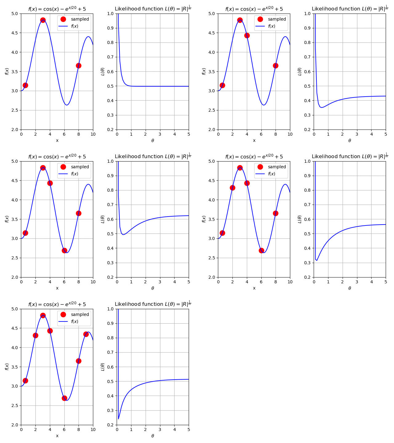
Due to some constraints (i.e. the model is too expensive or slow to compute), we can only have a small amount of samples (red circles). For inspection purposes, we decide to spend some of our “budget” and sample three points initially. Plotting this model we have:

Fig. 123 Plot of function (24). The blue line is the true behavior of the model.

Plotting the equation (21), we se that this initial sample of three points gives use a monotonic behavior (you could say it’s “plateuing”) for the likelihood function. Or in simpler terms, there is no clear discernible minimum. This will, likely, result in a poor fit.

Fig. 124 Initial plot of the likelihood (21) as function of the hyperparameters \(\theta\).

So what is the solution for this? We decide to spend a bit more of our budget and add four more samples to the fit. Again, we plot the results iteractively to demonstrate the effect:

Fig. 125 The effect of adding more samples to our surrogate.

As we can see, the more we add to the initial sample, the better is to find a minimum for (21).

Caution

In this case, we used a simple function for demonstration purposes. When dealing with way more complex models, the “budget” we mentioned earlier is the computational effort of the Kriging metamodel, since it has a \(\mathcal{O}(n^3)\) complexity, there is a trade-off between sample size and how satisfied we are with our surrogate.

However, now you may question: “With higher dimensions models, we can’t simply plot this function and do this analysis. So what should I do?”

The answer is simple. If you look closely at Fig. 125, you may notice that as \(\theta\) increases, the likelihood reaches its plateau. This behavior is due to that \(R\) (or (20)) tends to become an identity matrix with high values of \(\theta\) (i.e. there is no correlation). When this happens, (21) approximates to the variance \(Var(y)\) of the sample \(y\).

Therefore a simple way to examine our quality-of-fit is to test the following equation:

(25)\[\psi(\theta^*) < Var(y)\]

Important

If (25) is true at the optimal \(\theta^*\), then, probably, the fit is good enough for our purposes. Otherwise, the model is, most likely, a poor fit.