Indirect composition control of a Propene/Propane Distillation Column
The system depicted in Fig. 73 consists of the separation of propene from a binary mixture with propane in a 146 stage distillation column. [3] showed that the best set of self-optimizing controlled variables as single measurements for this system are the composition of propene in the distillate and bottom products at their respective optimum nominal values. However, because direct control of composition is known to be difficult due to unreliability and slow dynamics of online analyzers, it may be better to use indirect control which is when control of primary variables can be achieved by selecting secondary variables such that the setpoint error is minimized. Metacontrol can also handle indirect control formulations since they are simply a special case of the exact local method [13][15][2].

Fig. 73 Flowsheet of the propene distillation column.
The objective is to minimize the relative steady-state deviation in (1) [16].
where \(x_{\text{top,setpoint}}^{\mathrm{propene}} = 0.995\) and \(x_{\text{bottom,setpoint}}^{\mathrm{propene}} = 0.05\) [3], subject to
C-1: Reboiler duty \(\leq 80 GJ/h\)
using the reflux ratio and the distillate to feed ratio as available degrees of freedom.
The main process disturbances are [3]:
D-1: Feed propylene flowrate
D-2: Feed propane flowrate
D-3: Feed vapor fraction (\(\phi\))
A typical temperature profile for the C3 splitter is shown in Fig. 74 , and since temperature is easy to measure, some particular stage temperatures along the column were chosen as candidate controlled variables based on the slope criterion of [27]. It is then expected that temperatures close to the top are poor choices of measurements vis-a-vis the ones close to the bottom (considering a top-down stage numbering). Moreover, some flows and flow ratios were also considered as candidates (see Table 2).

Fig. 74 Temperature profile.
Variable (alias used in Metacontrol) |
Description |
|---|---|
bf |
Bottoms to feed ratio |
vf |
Boilup to feed ratio |
lf |
Reflux to feed ratio |
rrcv |
Reflux ratio |
dfcv |
Distilalte to feed ratio |
l |
Reflux rate \((kmol/h)\) |
v |
Boliup rate \((kmol/h)\) |
t8 |
Stage 8 temperature \((°C)\) |
t9 |
Stage 9 temperature \((°C)\) |
t10 |
Stage 10 temperature \((°C)\) |
t11 |
Stage 11 temperature \((°C)\) |
t12 |
Stage 12 temperature 4\((°C)\) |
t129 |
Stage 129 temperature \((°C)\) |
t130 |
Stage 130 temperature \((°C)\) |
t131 |
Stage 131 temperature \((°C)\) |
t132 |
Stage 132 temperature \((°C)\) |
t133 |
Stage 133 temperature \((°C)\) |
t134 |
Stage 134 temperature \((°C)\) |
t135 |
Stage 135 temperature \((°C)\) |
t136 |
Stage 136 temperature \((°C)\) |
With 20 candidate controlled variables and 2 degrees of freedom there are \(\binom{20!}{2!} = \frac{20!}{2!\times(20-2)!} = 190\) possible control configurations of single measurements, and the evaluation of all of these one at the time is a very tedious task. Fig. 75 and Fig. 76 shows the problem setup in Metacontrol.
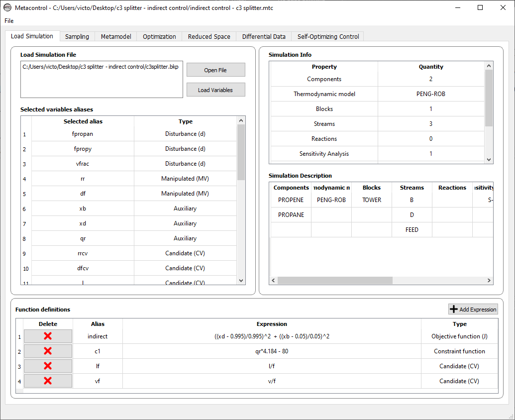
Fig. 75 Problem setup for the C3 splitter column process.
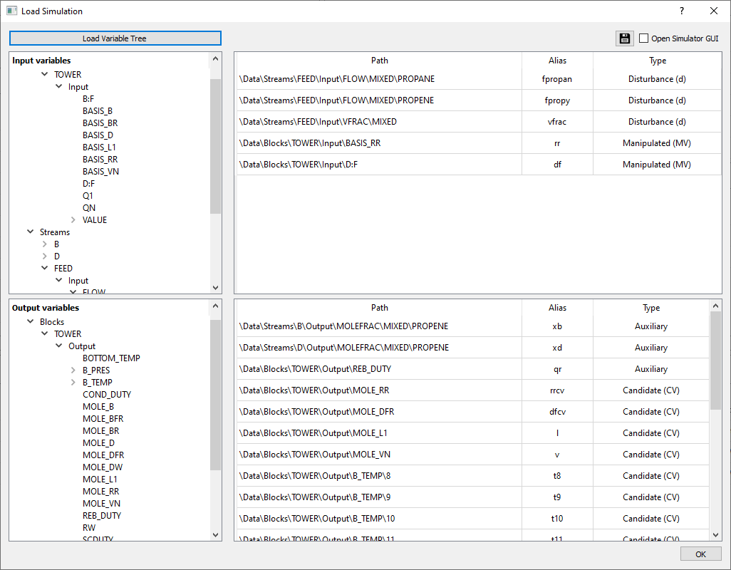
Fig. 76 Aspen Plus variable load for the C3 splitter column process.
A total of 60 initial points were sampled (Fig. 77) and refined by the algorithm of [6] in Metacontrol to find the optimal nominal operating point. Using a K-fold validation, it was observed that the quadratic regression polynomial (poly2) yielded the most accurate Kriging metamodel. This is indeed a valuable feature of Metacontrol for it systematically informs which regression model provides the most promising results. (Fig. 78- Fig. 80.)
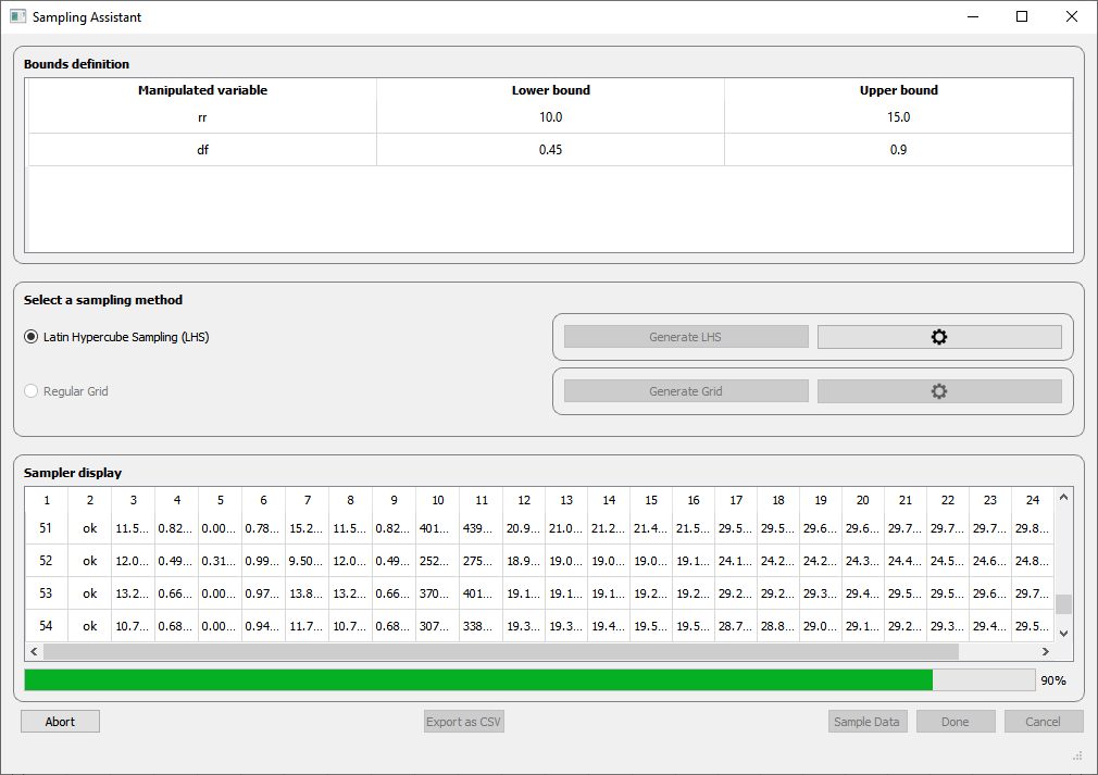
Fig. 77 Initial sampling for the C3 Splitter case study and the bounds considered.
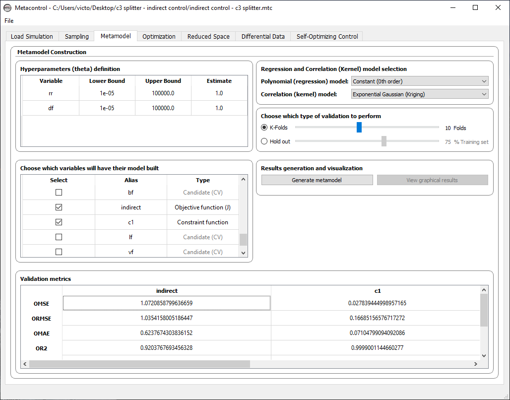
Fig. 78 K-fold validation metric for constant (poly0) regression model.
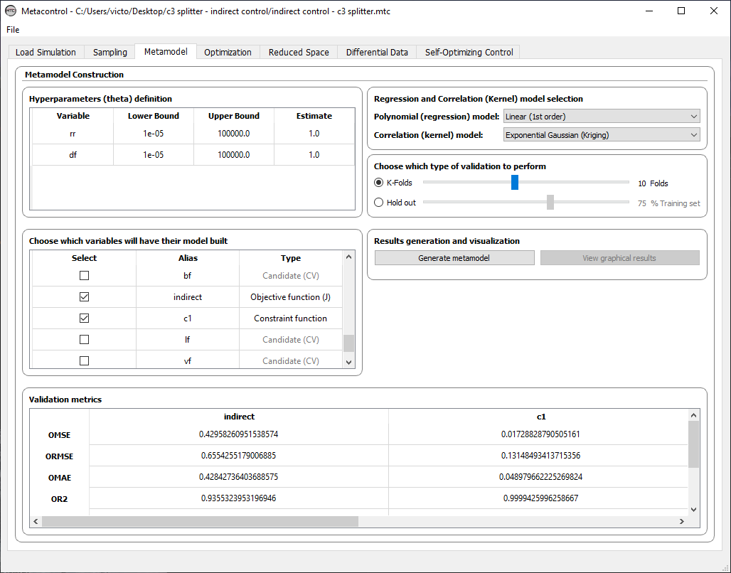
Fig. 79 K-fold validation metric for linear (poly1) regression model.

Fig. 80 K-fold validation metric for linear (poly2) regression model.
Fig. 81 reports the results of the optimization in Metacontrol. As there are no active constraints, two unconstrained degrees of freedom are left for self-optimizing control purposes. Table 3 shows that the optimization conducted in Aspen Plus matches the one in Metacontrol.
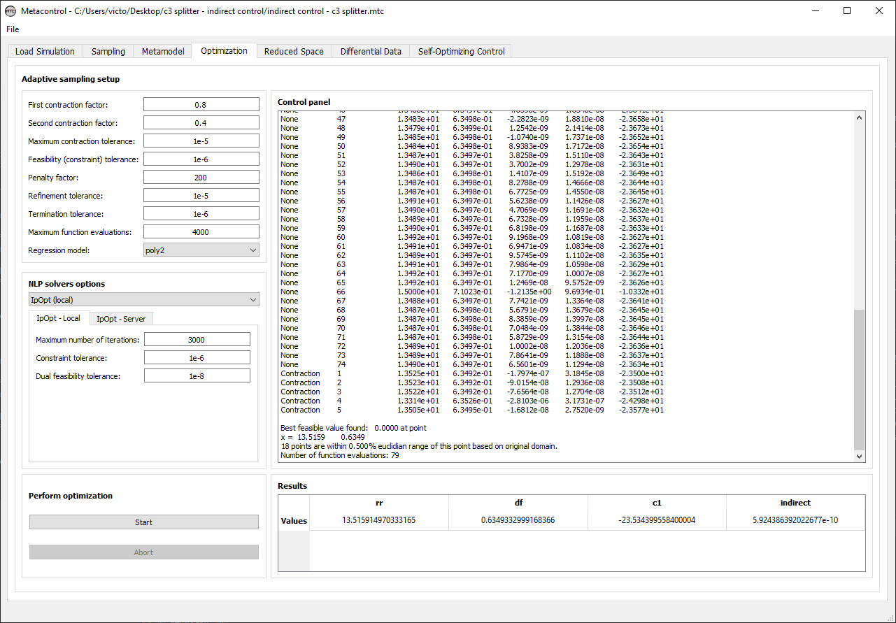
Fig. 81 Refinement algorithm log output.
Objective function |
Reflux Ratio |
Distallate to feed ratio |
|
Aspen Plus |
\(7.47 \times 10^{-15}\) |
13.5246 |
0.6349 |
Metacontrol |
\(5.92 \times 10^{-10}\) |
13.5159 |
0.6349 |
With no active constraints to be implemented in the process simulator, the reduced space Kriging metamodel was built using the same .bkp file of the optimization step (Fig. 82 and Fig. 83). Here the reduced space sampling was done within Metacontrol, reducing the need to navigate between applications.
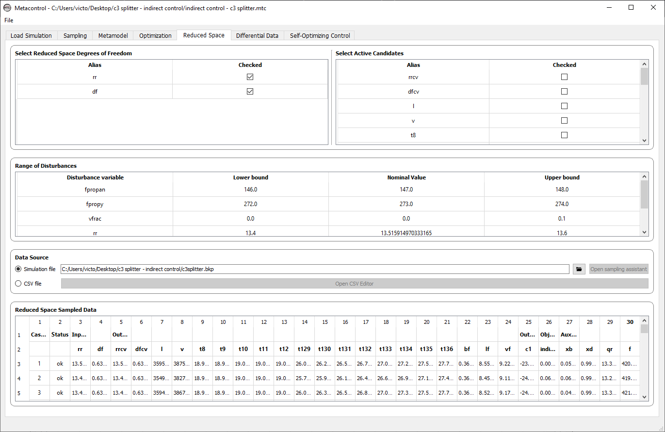
Fig. 82 Reduced space problem sampling using a .*bkp file.
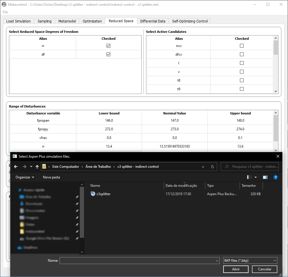
Fig. 83 Pointing to the .*bkp file location.
Hitting the “Open sampling assistant” button (1) in Fig. 84 opens the window (2) where the parameters of the sampling method can be set (3) and the data generated (4). The sampling can also be controlled (5), and the user can abort the process at any moment (6), or export the results as a .csv file (7).
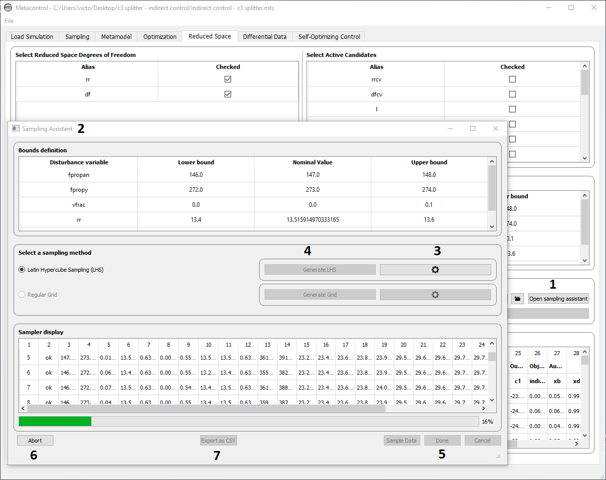
Fig. 84 Sampling assistant for the reduced space metamodel construction.
Gradients and Hessians for the self-optimizing control formulas are generated at the “Differential Data” tab of Figure Fig. 85. The gradients computed by Metacontrol were compared against the ones generated by the process simulator (Fig. 86). Not surprisingly they were virtually identical, which is an evidence of the robustness of the previously proposed methodology of [3] that is implemented in Metacontrol.
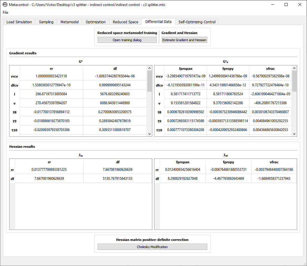
Fig. 85 Computation of derivatives in Metacontrol.

Fig. 86 Comparison between Aspen Plus and Metacontrol gradient results.
The magnitude of disturbances in this case were \(10\%\) for each component feed flow rate and \(10\%\) for the feed vapor fraction. The measurement errors were \(0.001\) for flow rates and flow ratios, and \(0.5°C\) for temperatures, a value that can realistically represent thermocouples and RTD sensor accuracies typically encountered in industry. Moreover, all 190 possible candidate controlled variables for the single measurement policy were considered. For linear combinations of measurements as candidate controlled variables, the 50 best subsets for each size were evaluated. This information was carefully specified in the “Self-Optimizing Control” tab of Fig. 87.
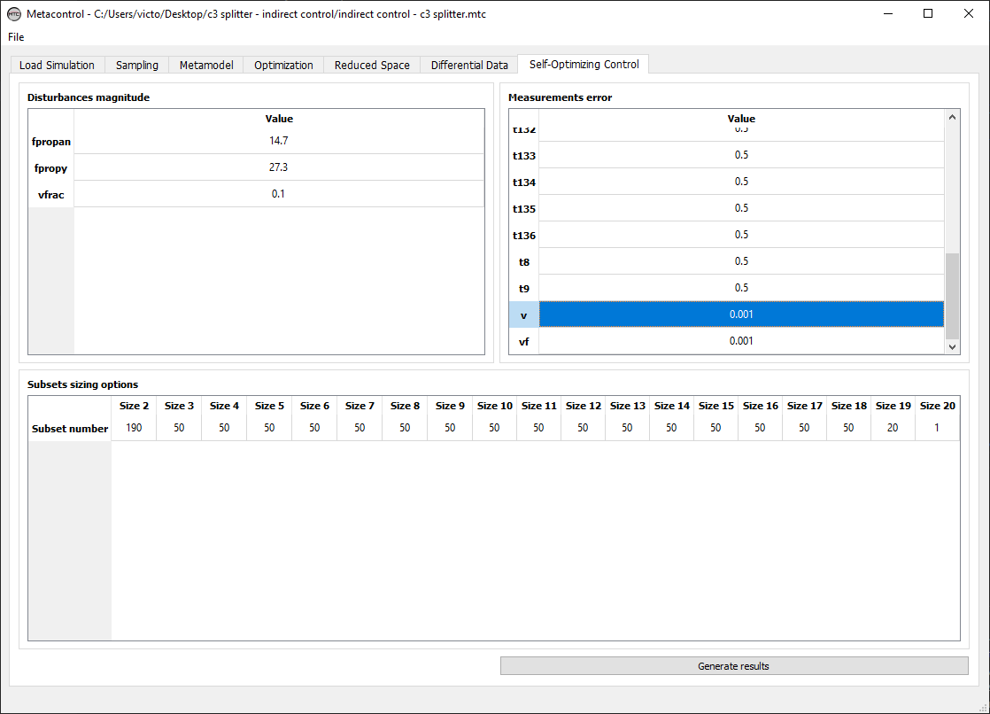
Fig. 87 Defining parameters for self-optimizing computations.
The results for the single measurement policy (Fig. 88) show that selecting sensitive temperatures and flow rates or flow ratios yields configurations capable of indirect controlling both distillate and bottom compositions with small incurred losses, while choosing less sensitive temperatures results in large setpoint deviations (Fig. 89) with substantial losses [3][14]. This result is also an instance of the slope criterion of [27] as a good starting assumption for deciding which variables should be controlled. The main difference is that the mathematical framework of Self-Optimizing Control incorporates these heuristics in a neat, systematic way.
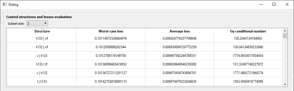
Fig. 88 Best sets of controlled variables for the single measurement policy showing small losses when selecting sensitive temperatures and flow rates or flow ratios.
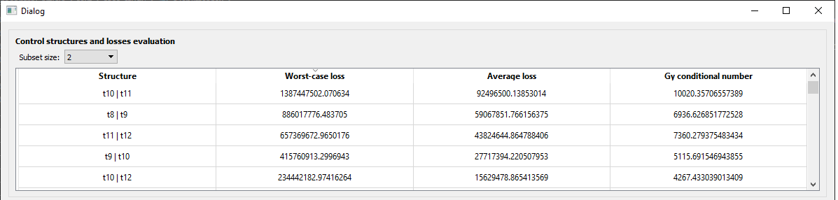
Fig. 89 Worst sets of controlled variables for the single measurement policy showing larger losses when selecting less sensitive temperatures. This is the same Fig. 88 sorted by worst-case losses in descending order.
Fig. 90-Fig. 93 show the results when linearly combining measurements for subsets of sizes 3, 6, 9, and 20 (using all measurements). Intuitively, the larger the number of measurements, the smaller the losses and the more complex the configurations with many measurements to combine, which shows a clear compromise between accepting greater losses and making the control scheme more tractable.
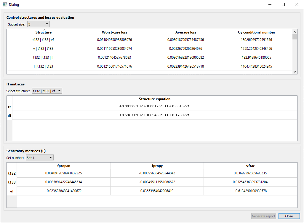
Fig. 90 Best sets of linear combinations of 3 measurements.
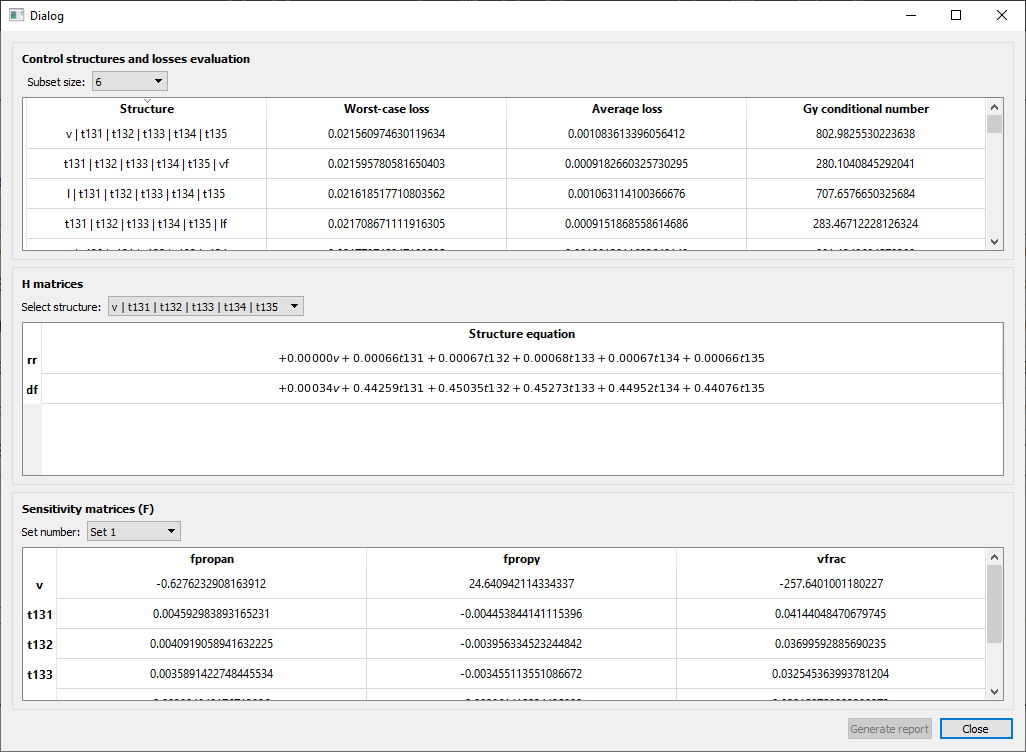
Fig. 91 Best sets of linear combinations of 6 measurements.
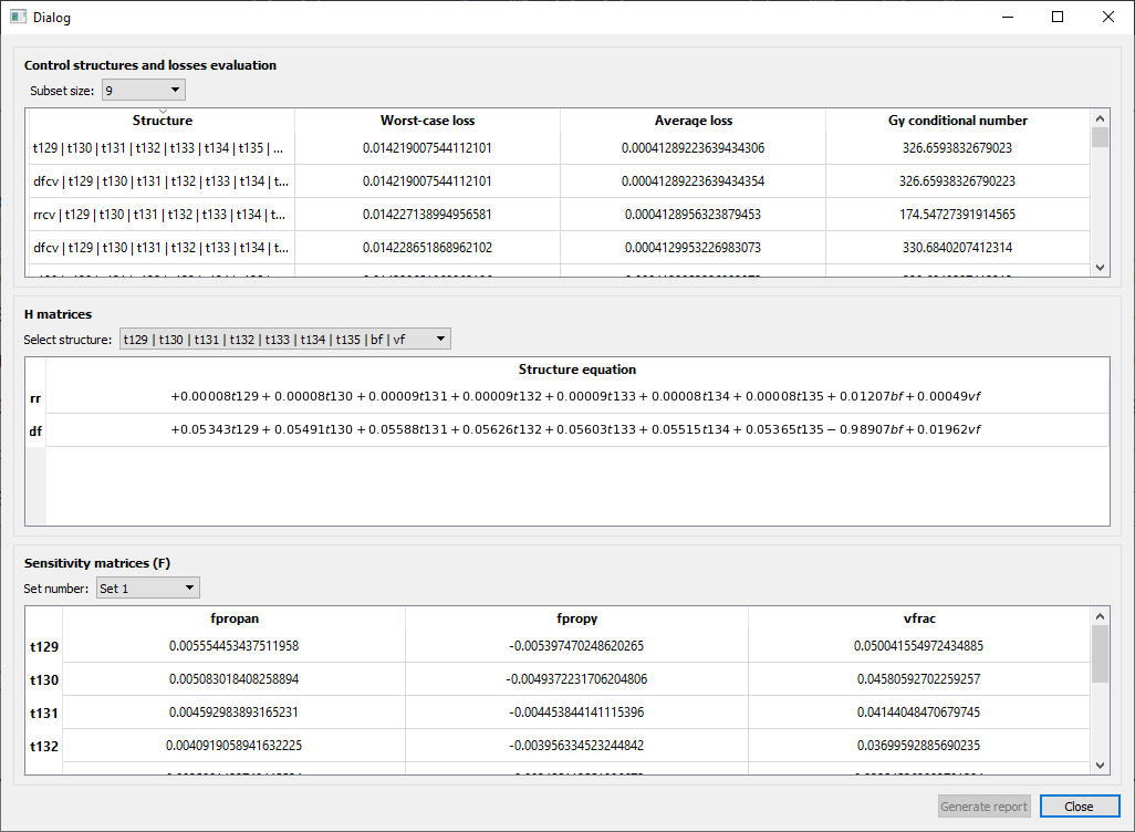
Fig. 92 Best sets of linear combinations of 9 measurements.
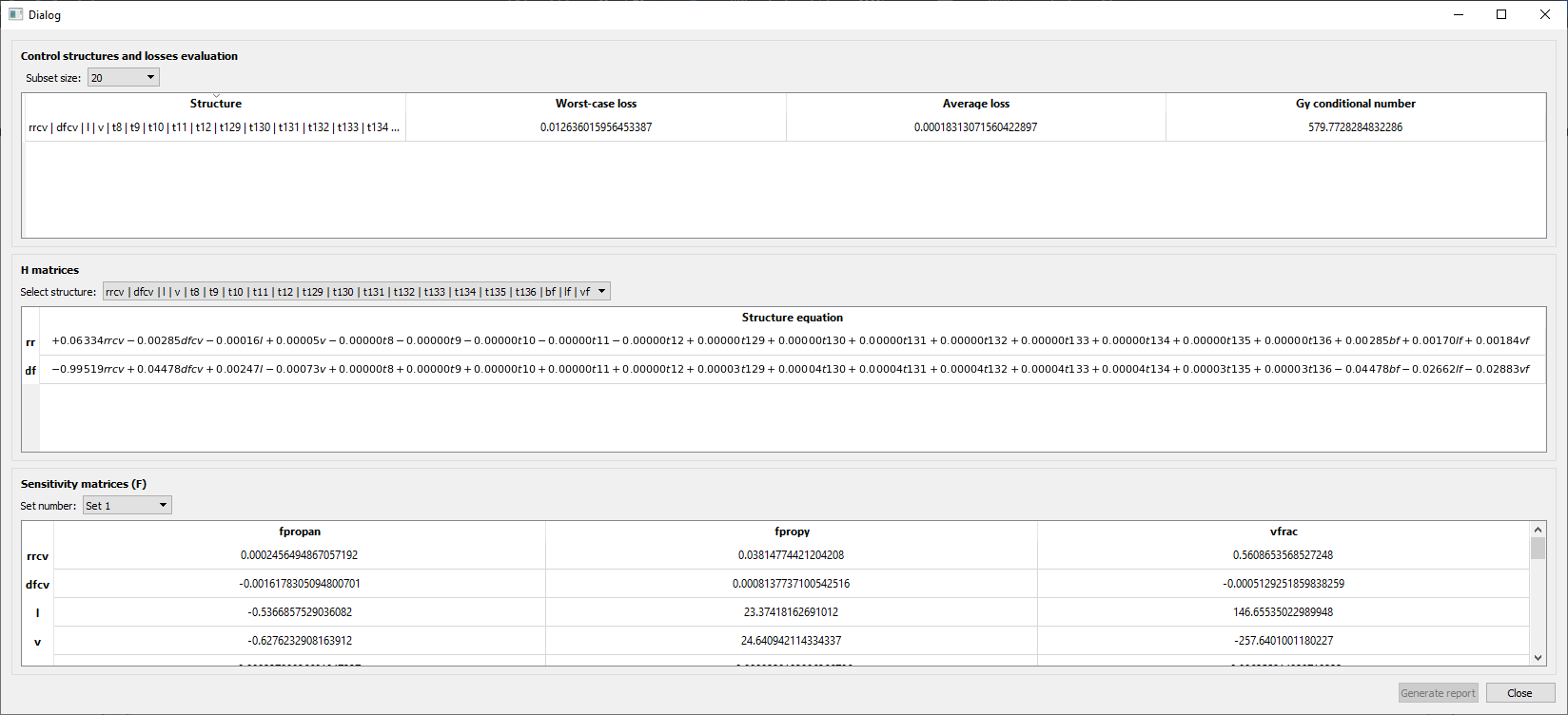
Fig. 93 Best sets of linear combinations of all measurements.
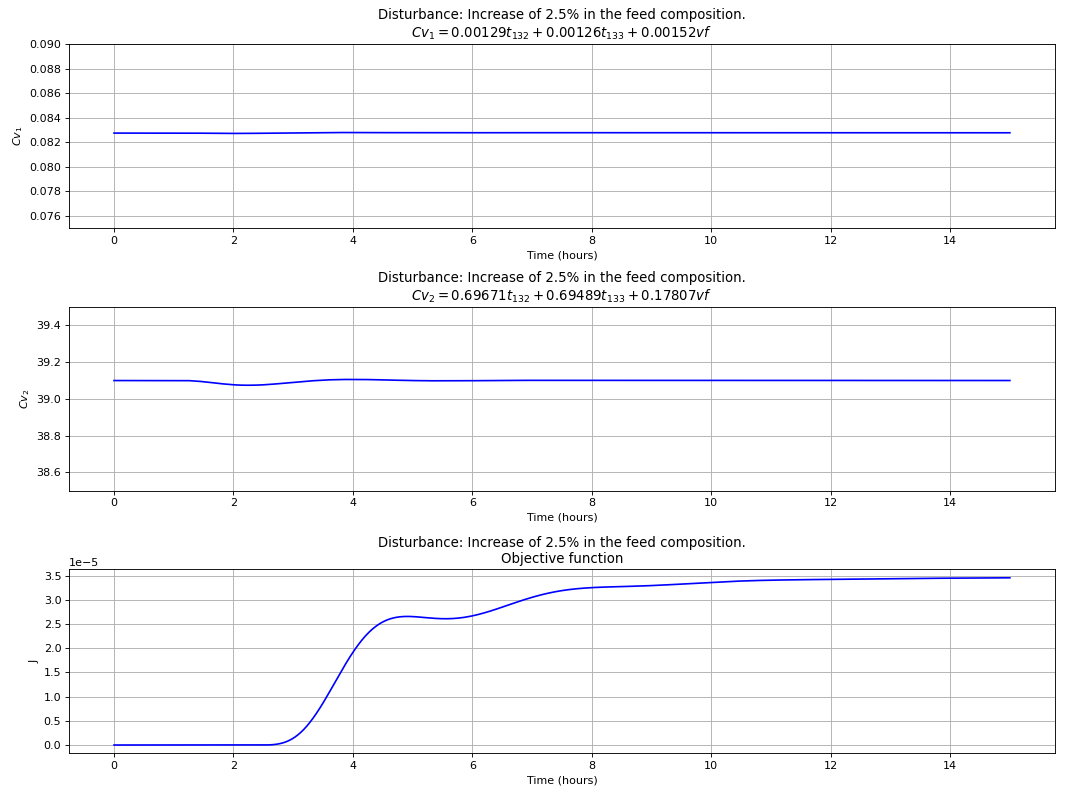
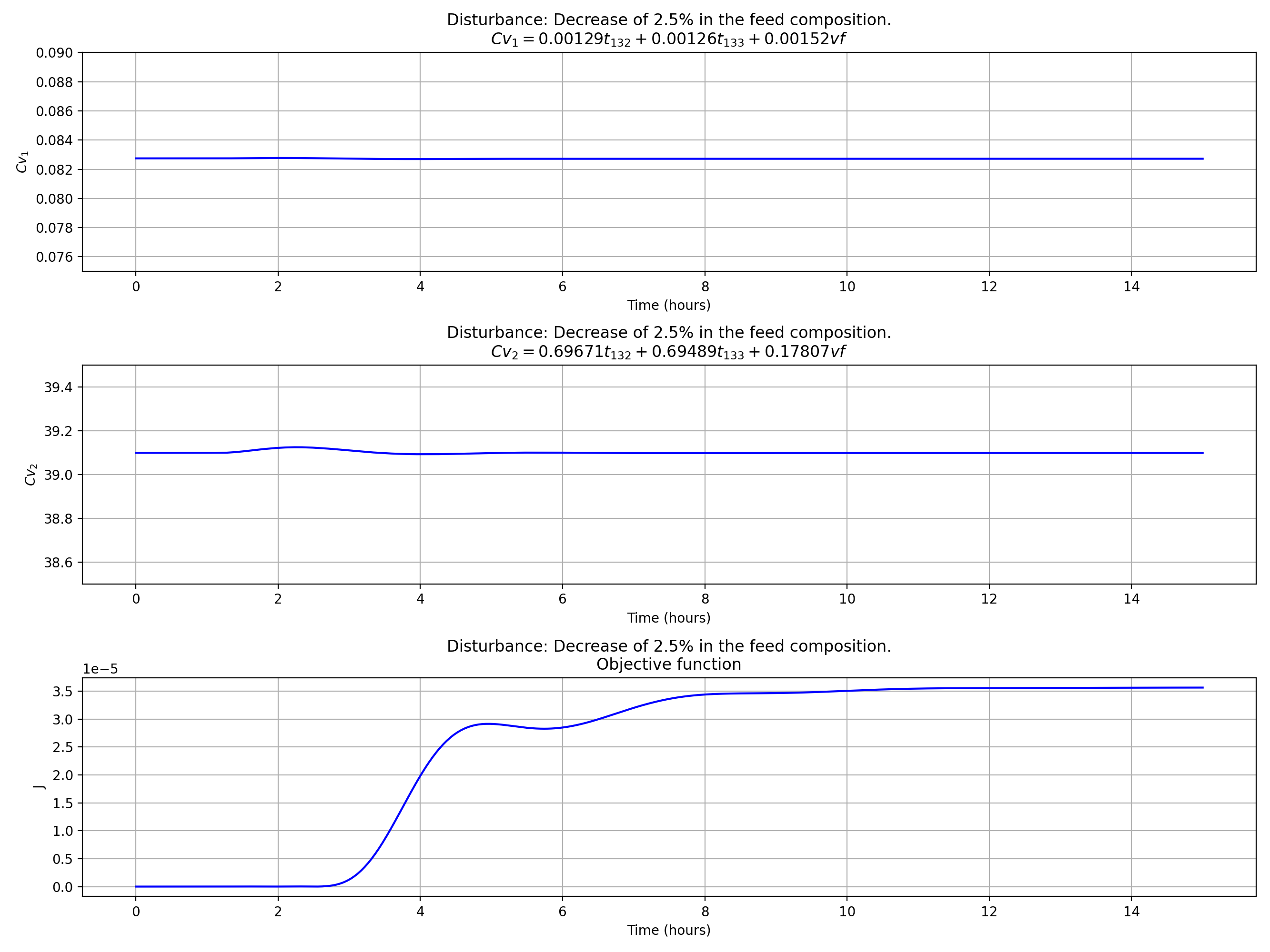
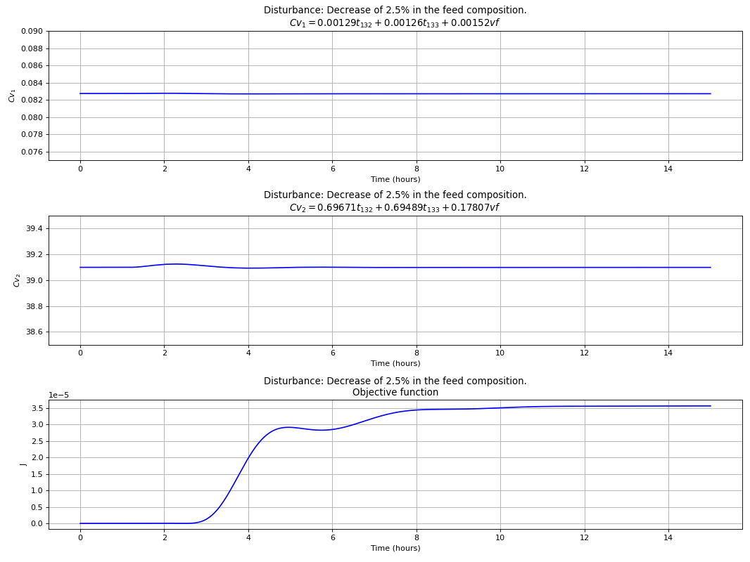
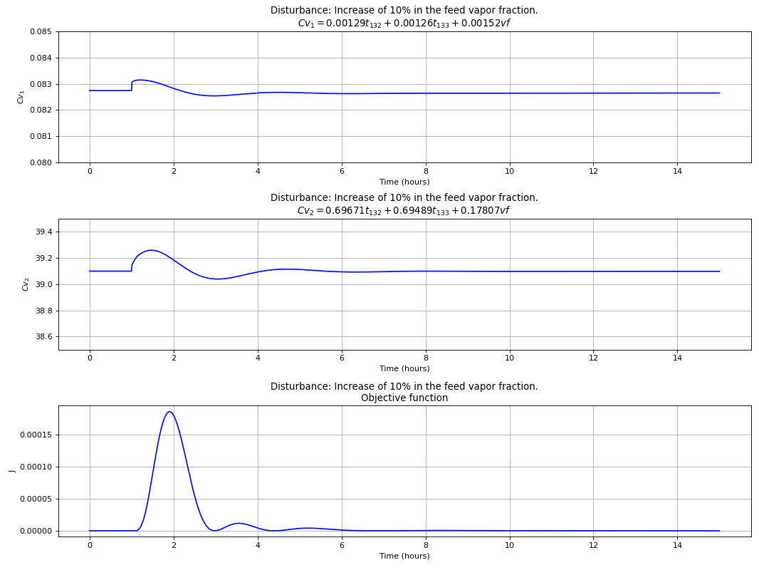
Dynamic simulations
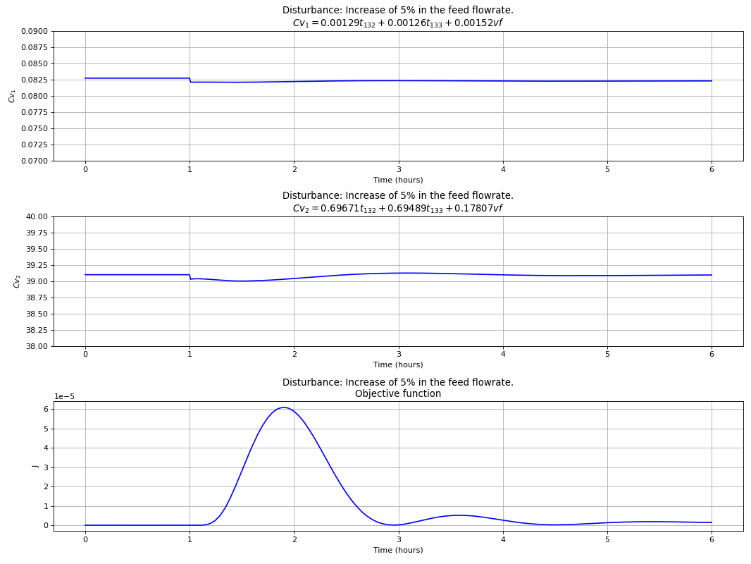
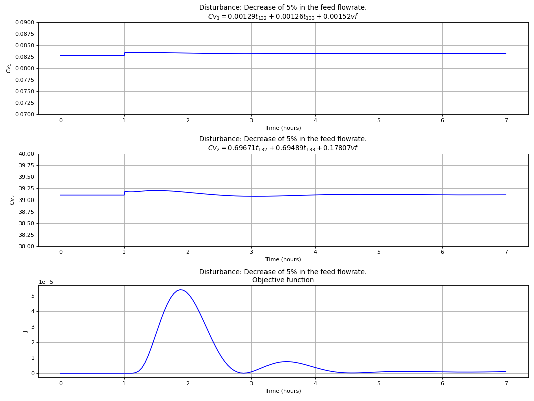
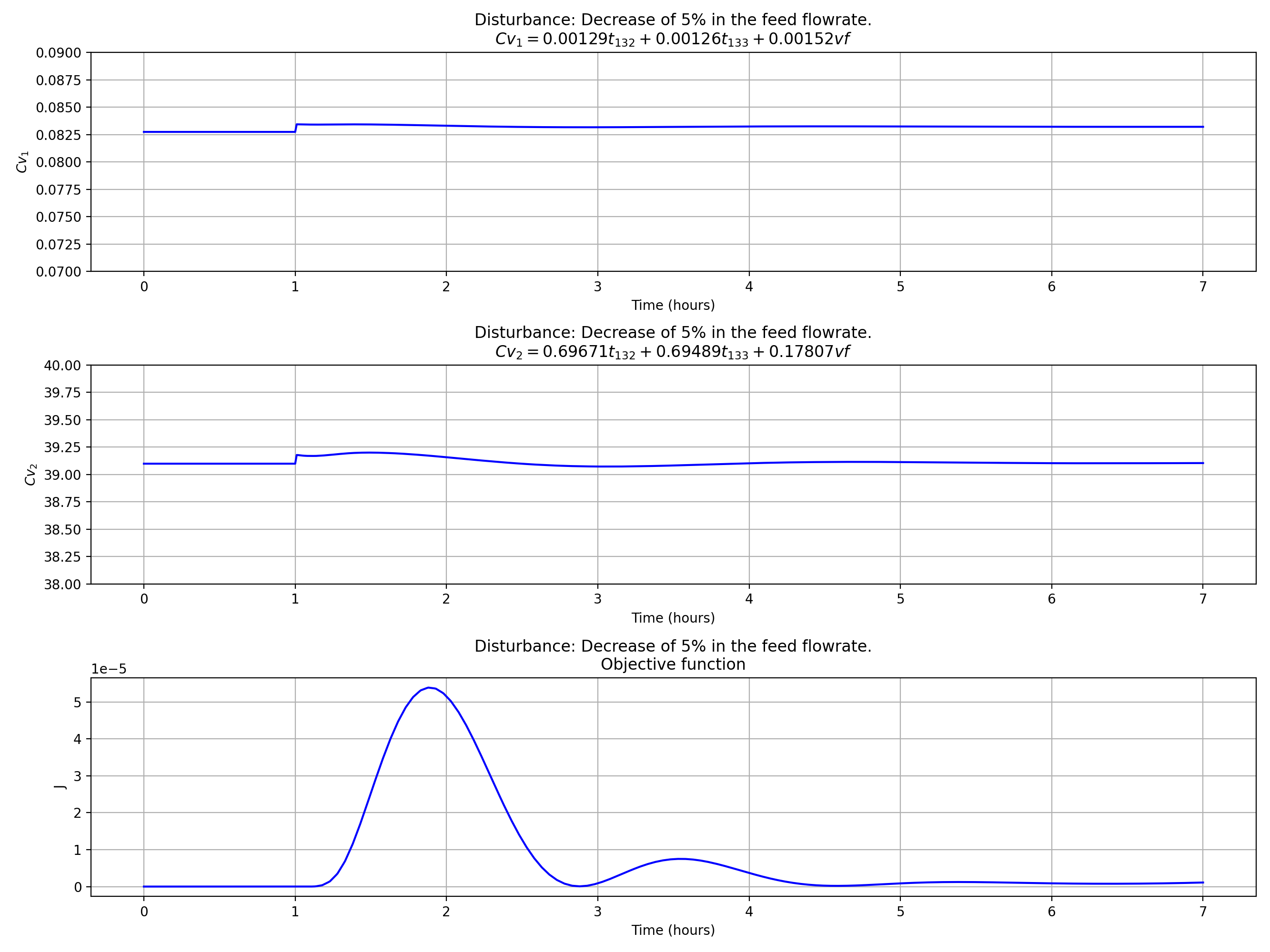
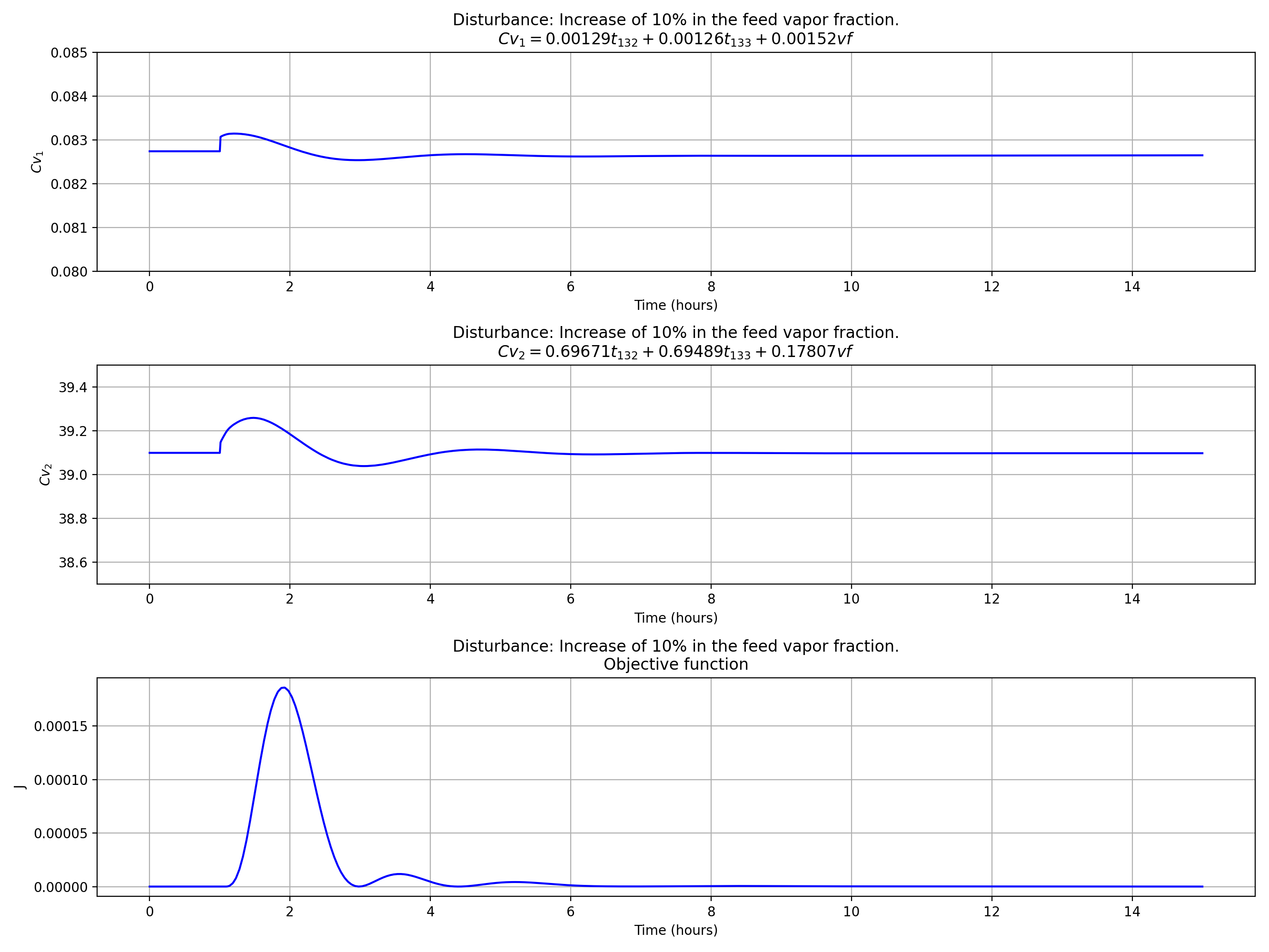
The best control structure that uses a linear combination of 3 measurements is chosen to evaluate the dynamic performance of this more complex control configuration for the C3-Splitter case study, where
The following plots clearly show that this choice is capable of dealing with disturbances in the composition of propene in the feed and total flow rate, while at the same time indirect controlling the primary variables. PI controllers tuned with the IMC rules and a process flowsheet depicting the control configuration in place is provided in Fig. 94.

Fig. 94 Control structure tested.


