Economic Self-Optimizing Control of a $C_{4}$ Isomerization process¶

Fig. 114 Flowsheet of the C4 isomerization process.¶

This case-study presented consists in a $C_{4}$ isomerization process, that aims to convert n-butane($n-C_{4}$) into isobutane ($i-C_{4}$). The latter can be used as an octane-enhancing gasoline blending agent, and also it is an precursor for isobutyl alcohol production [17]. The process described in this case-study it is based on the work of [17]: Base operating conditions and optimal operating ones. The idea of this case study is to depict to reader the second mode of operation that can be used in Metacontrol, described in when the optimal operating point it is known. This was implemented within because there is a plethora of papers and discussions over the several years that addresses the optimization of several processes ([17][18][9][4][12][24][32], just to name a few), and when one is dealing with economic plantwide control specially, there are several results that can be anticipated regarding active constraints.

Thus, it is understood that there is a relevant number of experienced researchers that have interest in using the the local methods derived by [13][2] in order to find self-optimizing variables (or linear combinations of measurements), but already know constraints that must be controlled on their particular applications, specially when this task can be done in a comprehensive software environment, which is the case for Metacontrol. In such cases, there is no need to used mode 1 from Metacontrol, and the user can simply build a metamodel of the reduced-space problem, merely providing the simulation file of the process with the active constraints already implemented, and sample the process using the unconstrained degrees of freedom, in order to generate the necessary high-order data, to finally obtain the most promising CV candidates.

The process flowsheet can be found on Fig. 114. The process was already optimized by [17] as stated before. Therefore, it was used the previously found optimal point from the aforementioned work, and it is described in Table 9. For this process, [17] kept the composition of n-butane on the bottoms of the purge column constant, and the other variables that are fixed were active constraints of the optimization problem: Either anticipated or calculated, except regarding the cooler temperature, that was alleged to have little impact on the objective function, and it was kept constant. Therefore, the aforementioned fixed composition will be considered as an unconstrained degree of freedom, differently from [17], and the reason is to evaluate if there is another variable that is easier to control than a composition that can be used in the control structure.

Table 9 C4 Isomerization process optimization summary.¶
Variable	Equation	Type
Objective Function [$\$/h$]	$J = - 9.83 \times Q_{furnace} - 4.83\times(Q^{reboiler}_{DIB-C}+Q^{reboiler}_{PURGE-C}) - 0.16\times (Q^{condenser}_{DIB-C} + Q^{condenser}_{PURGE-C}) - 32.5\times F_{C_4} + 42\times F_{i-C_4} + 22\times F_{i-C_5}$	Profit
Reactor Temperature Specification	$T_{\mathrm{reactor}}=200^{\circ} \mathrm{C}$	Active
DIB-C Boilup Constraint	$0 \leq V_{1} \leq 1.3$	Base case
PURGE-C Boilup Constraint	$0 \leq V_{2} \leq 1.5$	Base case
Furnace Constraint	$0 \leq Q_{\text {furnace }} \leq 1.3$	Base case
Reactor Pressure Specification	$P_{\mathrm{reactor}}=45$	Active
Cooling Specification	$T_{\mathrm{cooler}}=53^{\circ} \mathrm{C}$	Fixed

In Fig. 115, it can be seen that the only expression built for this problem was the economic objective function, due to the fact that the problem is already unconstrained (the active constraints are already known). Similarly to the first and second case studies, the user must identify the process disturbances, CV candidates and degrees of freedom (Fig. 116).

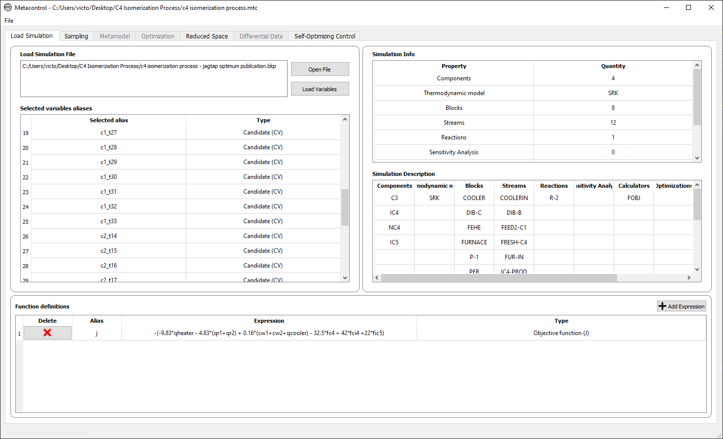
Fig. 115 C4 Isomerization process - loading simulation. The cooling water price is positive due to signal convention inside the process simulator - heat removed from the system has a negative sign.¶

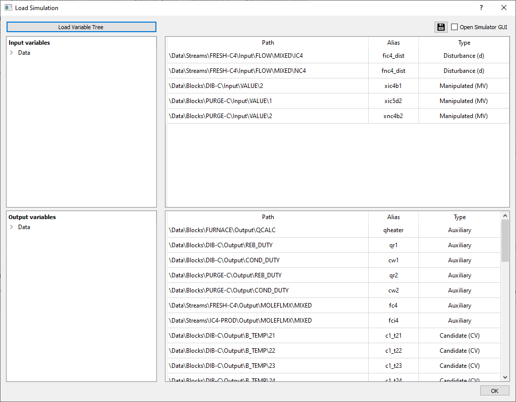
Fig. 116 C4 Isomerization process - loading variables.¶

For the expected disturbances, the values come from [17], and disturbances for the amounts of isobutane and textit{n}-butane in the feed were considered, with a range of $10\%$ of the nominal values. However, instead of considering the compositions, the values of the individual component flow rates were used in the design of experiments. Regarding CV candidates, sensitive temperatures at the optimal operating point were inspected for both columns, and the most sensitive ones were considered as CV candidates. The full list of CV candidates can be seen in Table 10.

Table 10 CV Candidates for $C_{4}$ Isomerization process.¶
Variable (alias used in Metacontrol)	Description
c1_t“x’	1st column stage X temperature (stages 21-33) $(°C)$
c2_t“x’	2nd column stage X temperature (stages 14-20) $(°C)$
x_ic4_b1	1st column $i-C_{4}$ bottoms composition
x_ic5_d2	2nd column $i-C_{5}$ distillate composition
x_nc4_b2	2nd column $n-C_{4}$ bottoms composition
c1_v	1st column boilup rate $(kmol/h)$
c2_v	2st column boilup rate $(kmol/h)$
c1_l	1st column reflux rate $(kmol/h)$
c1_l	2nd column reflux rate $(kmol/h)$

50 points were sampled with an amplitude of $\pm0.5\%$ around the optimal point (Fig. 117), and the gradients and hessians could be extracted (Fig. 118). Lastly, Similarly as the previous cases, the implementation error for temperatures was considered as $0.5(°C)$, $10^{-3}$ for flow rates and $10^{-6}$ for compositions. All the aforementioned data was inserted inside Metacontrol, as can be seen in Fig. 119.

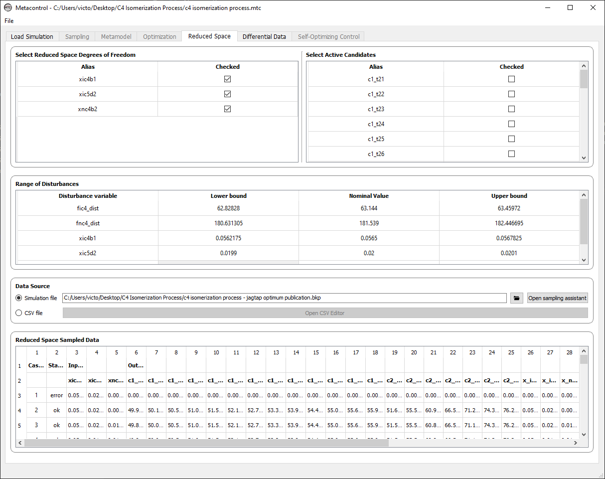
Fig. 117 C4 Isomerization process - loading variables.¶

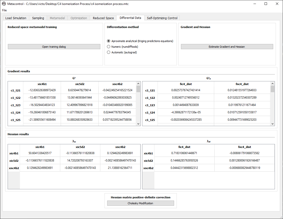
Fig. 118 C4 Isomerization process - High-order data obtainment.¶

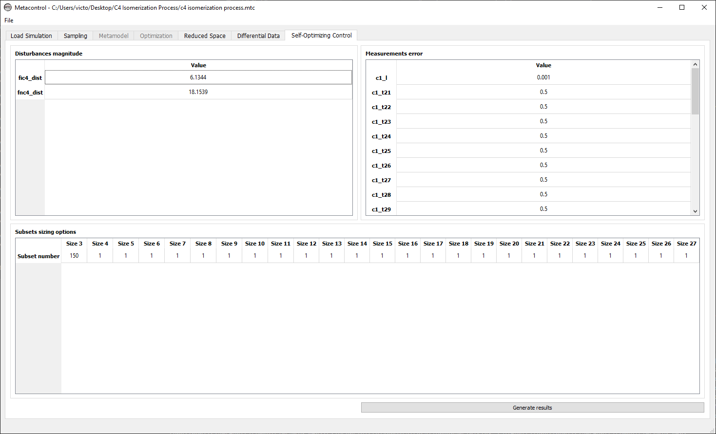
Fig. 119 C4 Isomerization process - Self-Optimizing Control input.¶

For the sake of brevity only the single measurement policy was considered in this analysis. Fig. 120 shows that, not surprisingly, the control of sensitive temperatures and the composition of the pollutant (in this case, $i-C_{5}$), yielded the lowest losses. However, keeping temperatures and flow rates with constant setpoints instead of using compositions are also promising control structures, as can be seen in Fig. 121

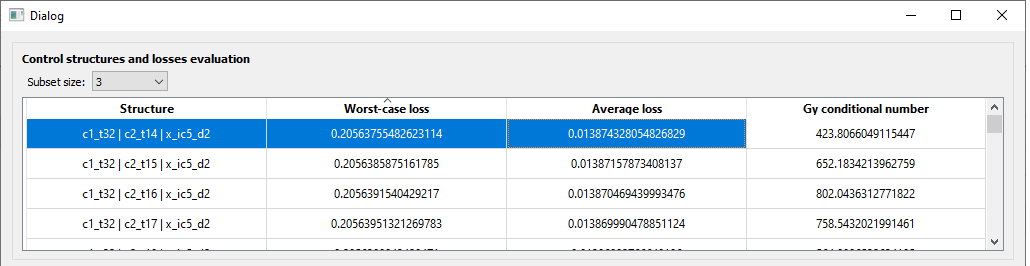
Fig. 120 C4 Isomerization process - Single measurements policy: Best CV candidates.¶

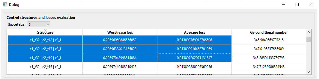
Fig. 121 C4 Isomerization process - Single measurements policy: Best CV candidates not using compositions.¶

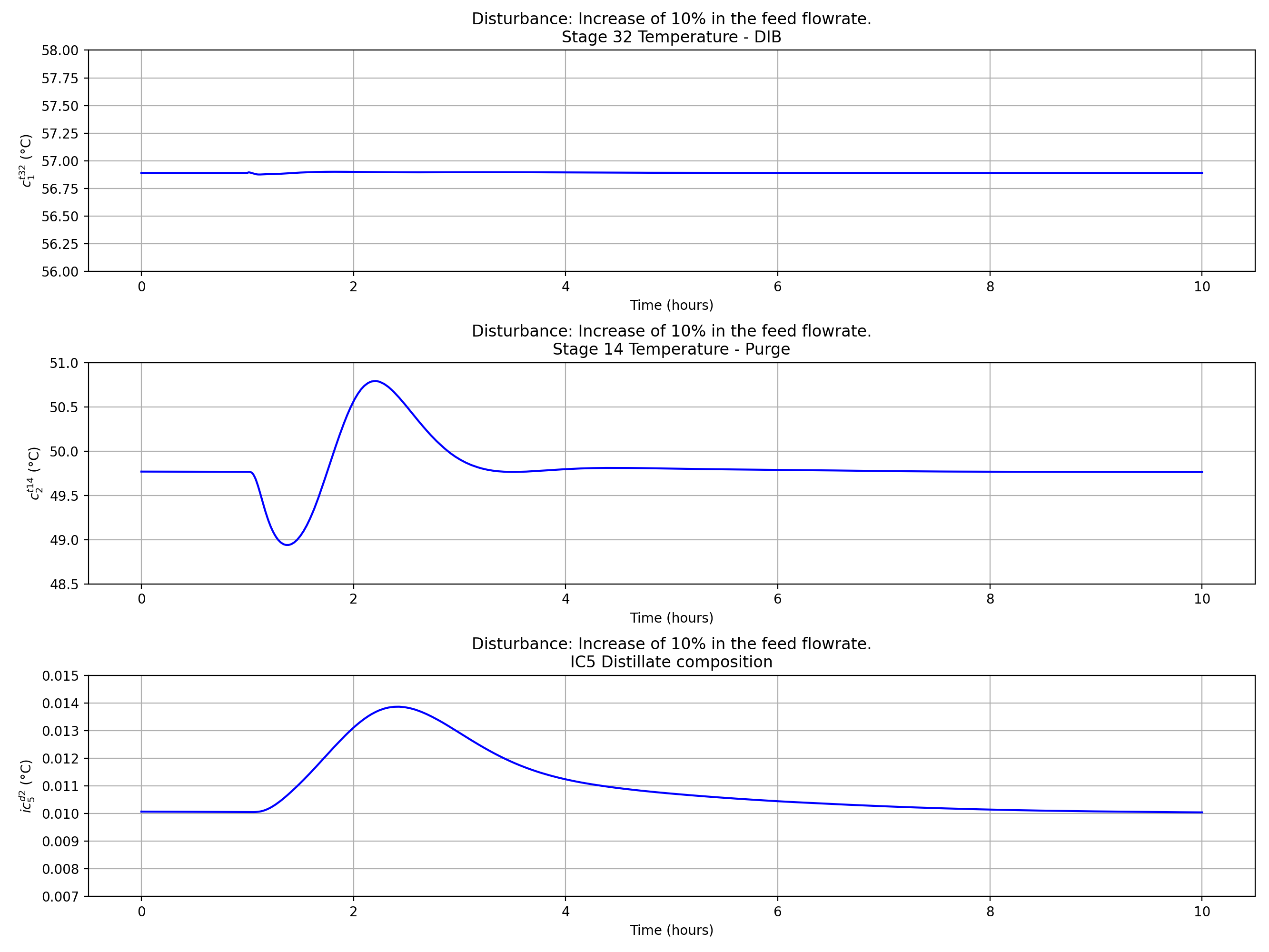
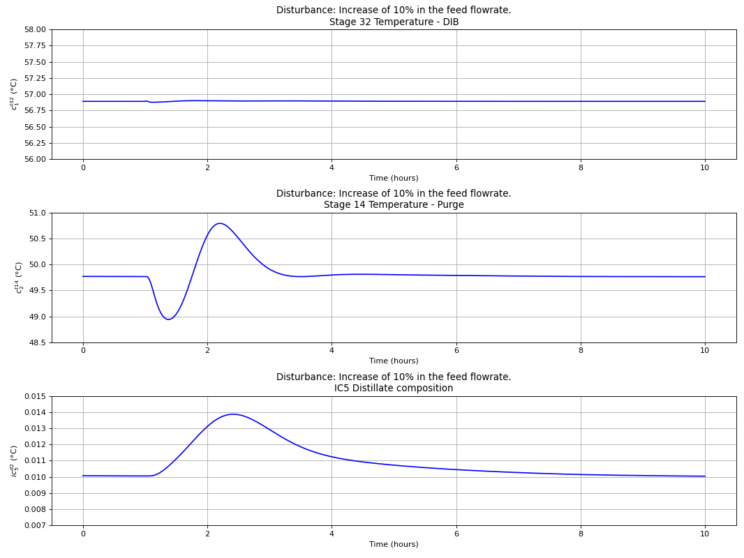
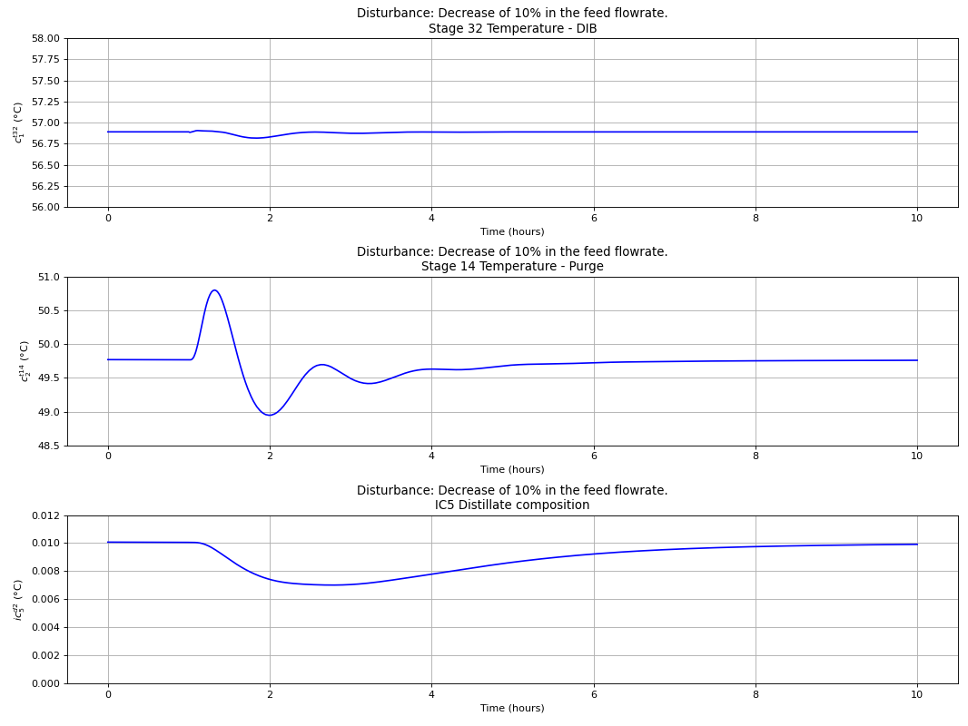
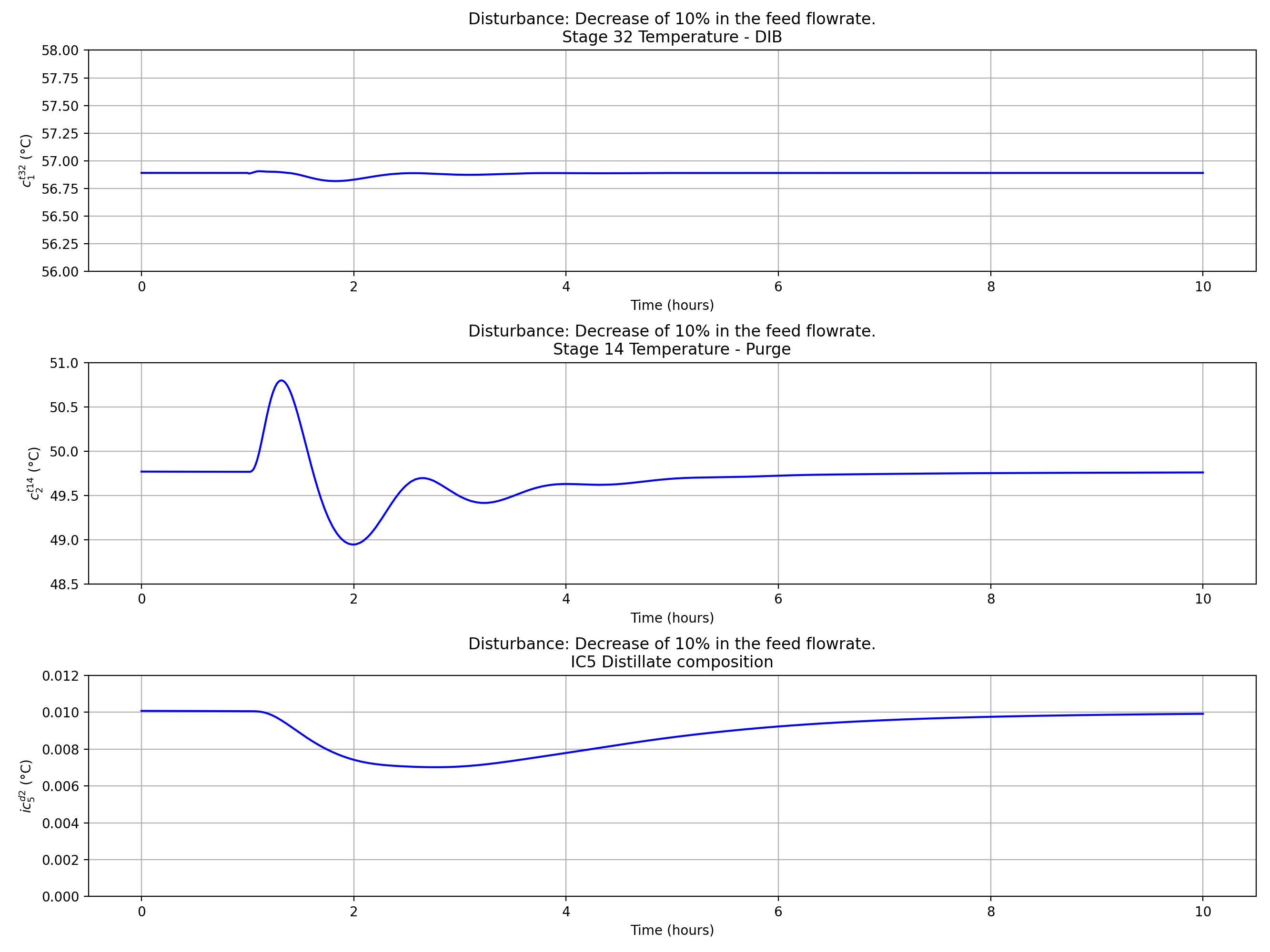
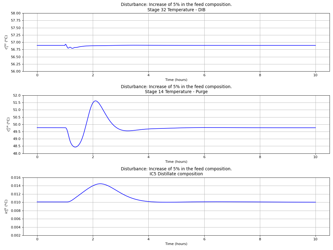
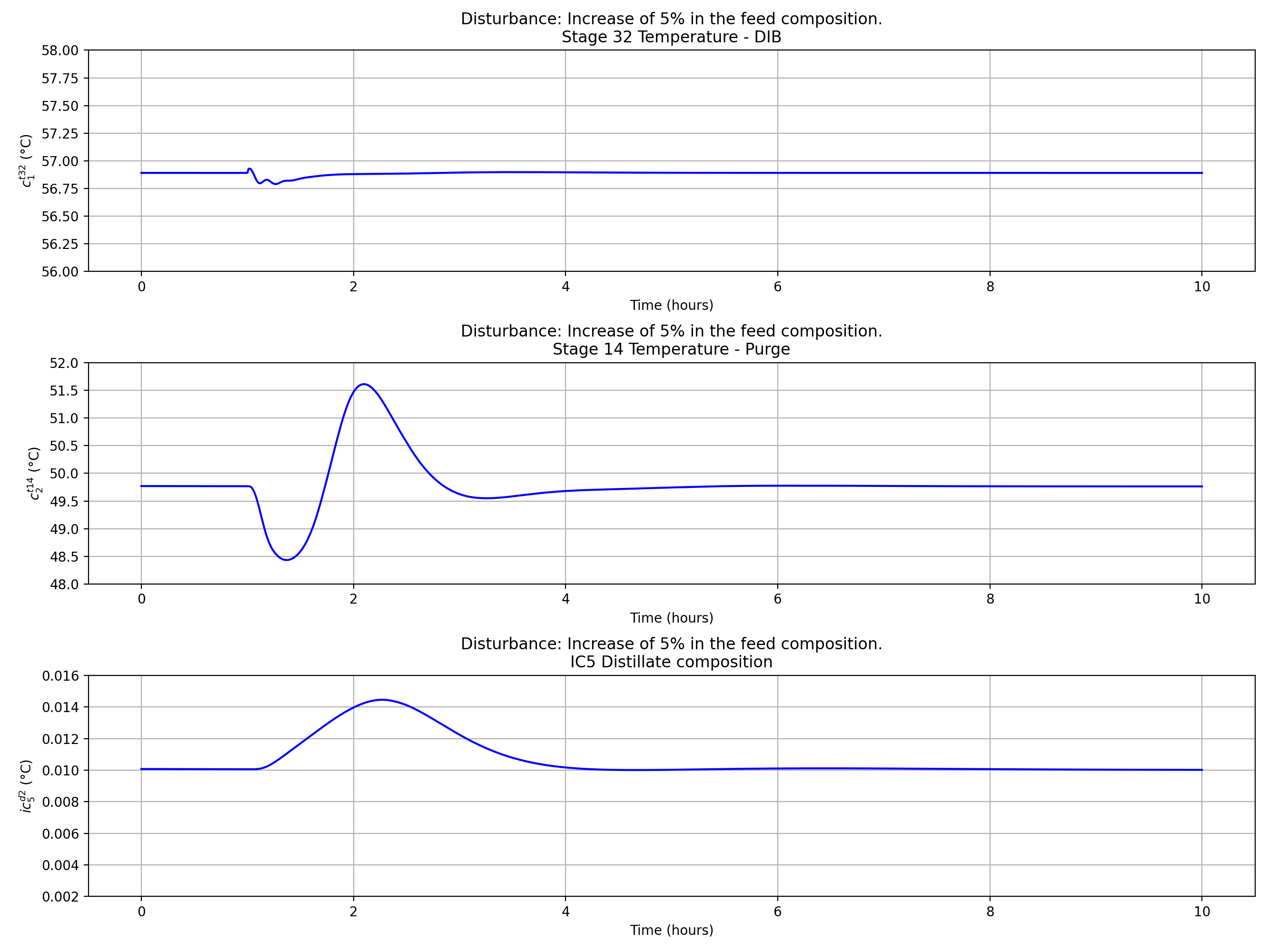
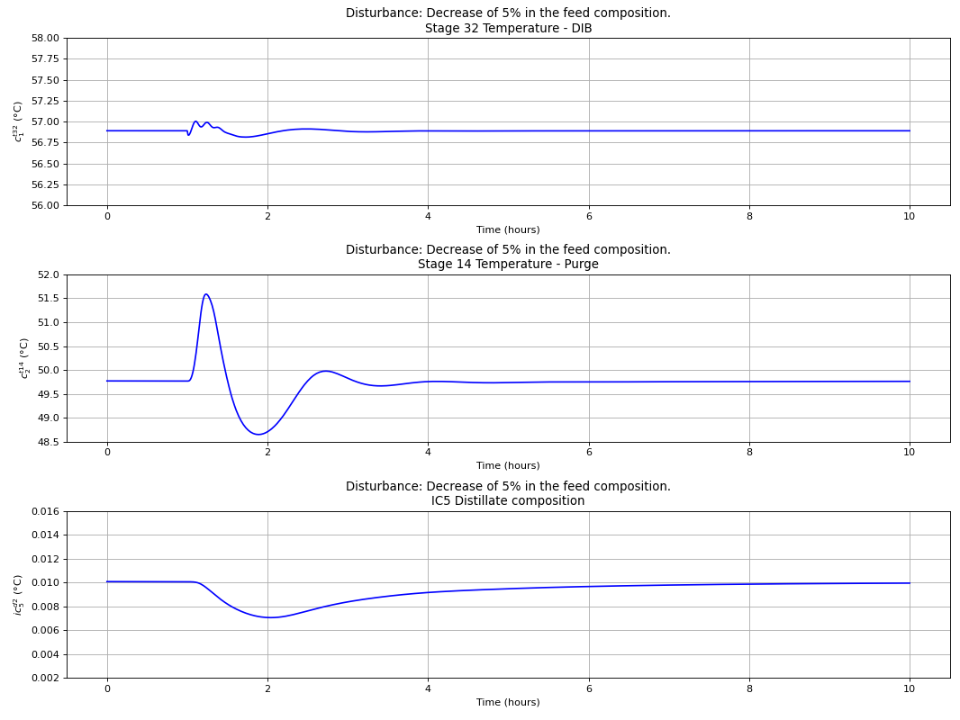
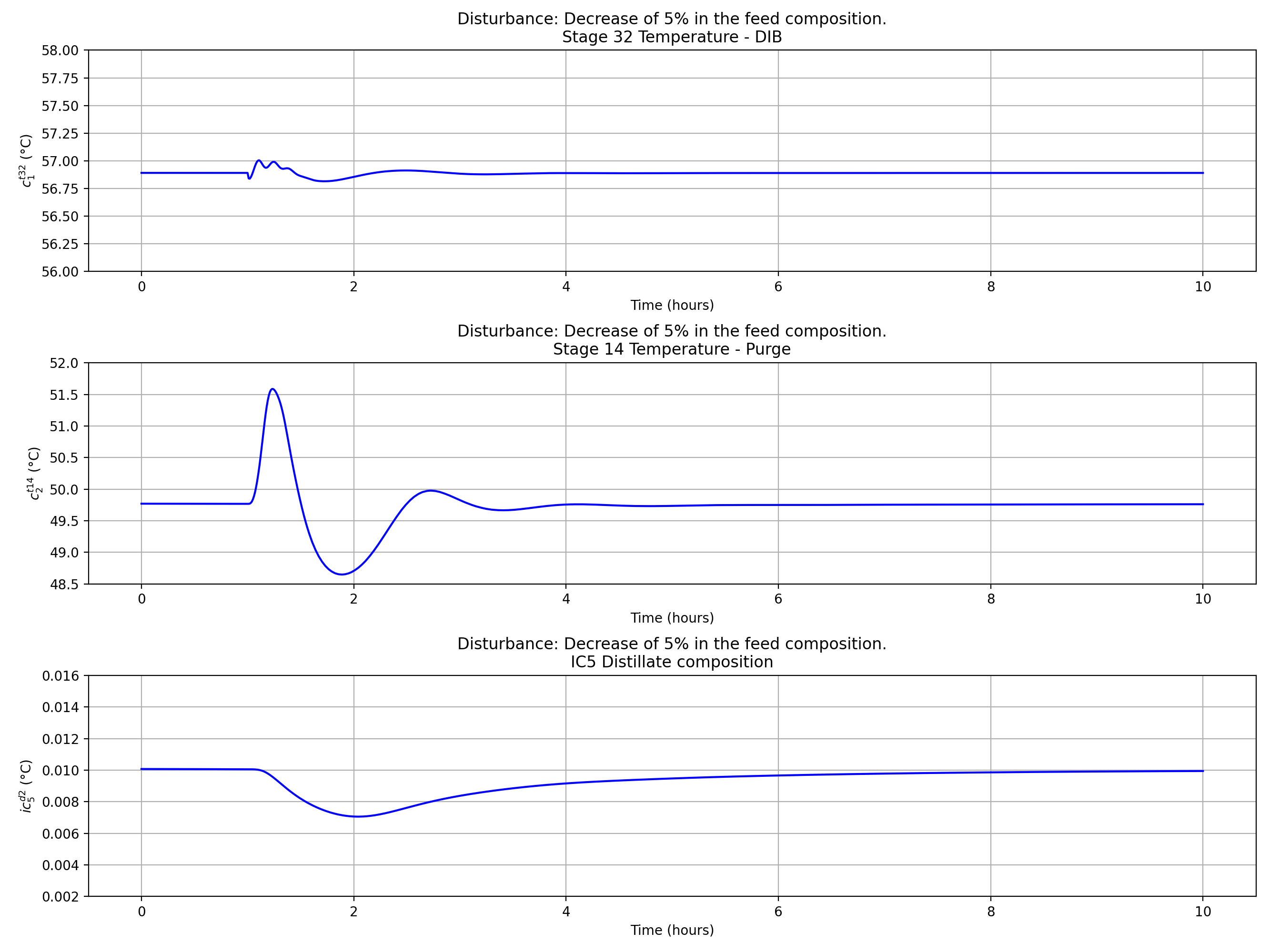
Dynamic simulations¶

Using the best single measurement policy of Fig. 120, the dynamic evaluation of the $C_{4}$ isomerization process was performed to prove the robustness of the SOC-based control structure. The controllers were tuned with the IMC tuning rules and disturbances on the feed flow rate and n-butane feed composition were made, with the results depicted in the next four figures. A process flowsheet depicting the control configuration in place is depicted in Fig. 122.