Economic Self-Optimizing Control of a \(CO_{2}\) Compression and Purification Unit

Fig. 95 Flowsheet of the CPU process.
The process consists in a \(CO_2\) compression and purification unit (CPU) that uses phase separation to produce purified \(CO_2\) from oxy-fuel combustion. This process is one of several capable of reducing the greenhouse effects on climate change [19] and it is based on the prototype proposed by the International Agency Greenhouse Gas (IEAGHG) R&D program study [10]. The modeling of the process depicted in Fig. 95 is inspired on the work of [24] and [19] and was implemented in Aspen Plus. Flue gas is compressed by a three-stage after-cooled compressor (MCC) and then sent to the first multi-stream heat exchanger (E1) where it is cooled to \(-24.51°C\) before separation in separator F1, the bottom of which consists of the first product stream. The top stream from F1 is the feed to the multi-stream heat exchanger (E2) where it is cooled to \(-54.69°C\) before going to separator F2, the bottom of which consists of the second product stream that is compressed in C. The top stream from F2 is discarded as vent. Both \(CO_2\) product streams and the vent gas are reheated on the multi-stream heat exchangers, and the \(CO_2\) product streams are mixed and sent to storage.
The objective is to reduce specific energy consumption by minimizing the cost function in (2) [24]
where \(W_{\mathrm{MCC}}\) and \(W_{\mathrm{C}}\) are the energy consumption of the compressors, and \(F_{\mathrm{CO}_2}\) is the \(CO_2\) feed flow rate.
The constraints to the process are [19][24][10]:
C-1: \(CO_2\) recovery rate \(\geq 90 \%\)
C-2: \(CO_2\) purity on product stream \(\geq 96 \%\)
C-3: Temperature of F2 bottom stream \(>-56.6°C\)
C-1 is an environmental requirement [24] to guarantee reduced \(CO_2\) atmospheric emissions [34][5], C-2 is a product specification used to prevent excessive energy consumption [29], and C-3 is there to avoid \(CO_2\) solidification in the pipeline since that bound corresponds to the \(CO_2\) three-phase freezing point [29][23].
The main disturbances to the process are [24]:
D-1: Flue gas flow rate
D-2: \(CO_2\) concentration in the flue gas
D-1 and D-2 are the result of the oxy-fuel combustion boiler island [24], given the variations on the boiler operation. The amplitude of variation was taken to \(\pm 5 \%\) of the base-case in both disturbances [24][19].
There are four steady-state degrees of freedom [24][19]
MCC outlet pressure (bar)
MCC outlet temperature \((°C)\)
F1 temperature \((°C)\)
F2 temperature \((°C)\)
Table 4 lists the candidate controlled variables considered for this case.
Variable (alias used in Metacontrol) |
Description |
|---|---|
mccp/mccpout |
Compressor outlet pressure (bar) |
mcct/mcctout |
Compressor outlet temperature \((°C)\) |
f1t/f1tout |
F1 temperature \((°C)\) |
f2t/f2tout |
F2 temperature \((°C)\) |
s8t |
S8 stream temperature \((°C)\) |
fco2out |
\(CO_{2}\) product flowrate \((t/h)\) |
xco2out |
\(CO_{2}\) product molar fraction |
co2rr |
\(CO_{2}\) recovery rate |
With 4 degrees of freedom and 8 candidate controlled variables there are \(\binom{8!}{4!} = \frac{8!}{4!\times(8-4)!} = 70\) possible control configurations for the single measurement policy, and the evaluation of each, one at a time, is definitely a tedious task especially if the procedure is not automated. That is exactly when Metacontrol is most needed.
The first step is to populate Metacontrol with the necessary process variables from the model in Aspen Plus using the COM interface. Fig. 96-Fig. 97 illustrate the process of loading a *.bkp Aspen Plus file, selecting the relevant variables, and creating aliases. Note that the *.bkp file must be compatible with the Aspen Plus version being used. The main window of Fig. 96 displays relevant information on the simulation in Aspen Plus such as block and stream names, flowsheet options (optimizations, sensitivities, calculators), the selected chemical species, and the thermodynamic package used.
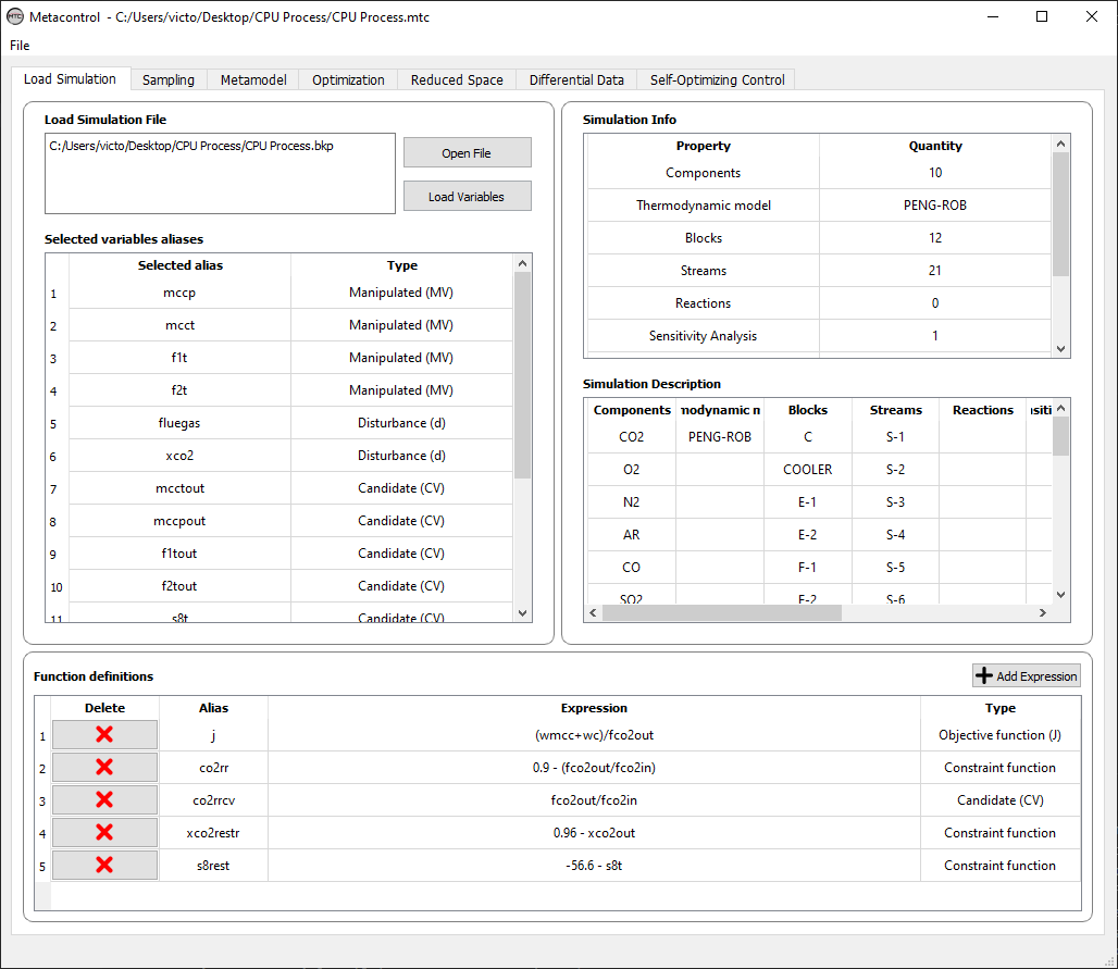
Fig. 96 Metacontrol main screen with the \(CO_2\) CPU process simulation file loaded. Note the vast display of information of the simulation from Aspen Plus.
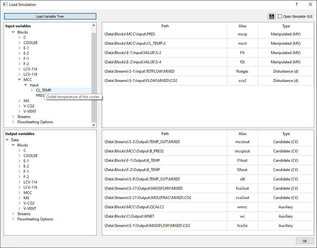
Fig. 97 Loading variables for the \(CO_2\) CPU process from Aspen Plus simulation and creating aliases. At the top right corner of this screen the user is able to select the option to reveal the GUI from Aspen Plus. This features allows for the inspection of the flowsheet in the process simulator to check for any stream or block name. Hovering the mouse over a COM variable on the GUI brings its description.
After selecting the relevant variables and define their types in the window of Fig. 97 the user can go back to the main screen where expressions can be created for the objective function, candidate controlled variables and constraints using the variables from the process simulator. Fig. 96 also shows the construction of such expressions for the \(CO_2\) CPU process using the auxiliary variables selected in Fig. 97.
The user can then generate the design of experiments (DOE) to build the Kriging responses of the objective function, candidate controlled variables, and process constraints (Fig. 98-Fig. 100). The ranges for each decision variable for the \(CO_2\) CPU process were taken from [19], which are automatically included as additional constraints to the problem formulation.
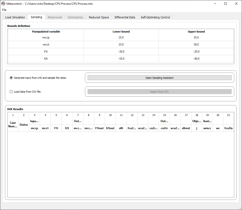
Fig. 98 Metacontrol sampling panel. The user can perform the sampling using the process simulator or importing a *.csv file.
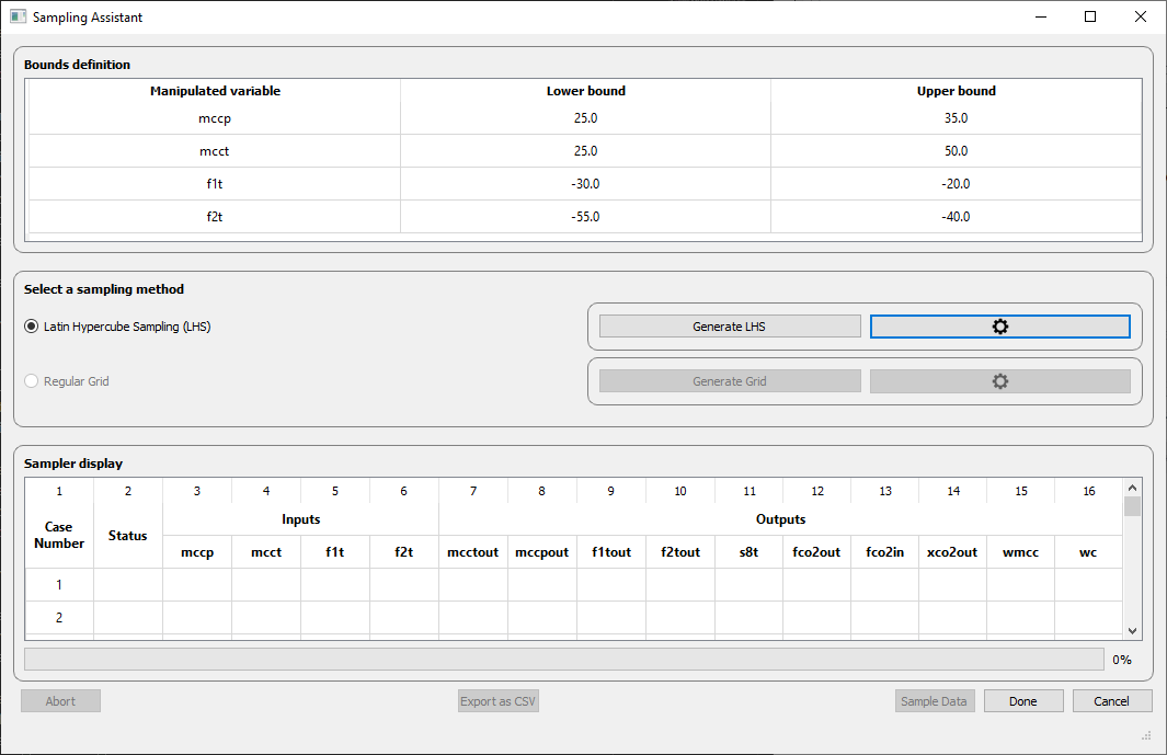
Fig. 99 Metacontrol sampling assistant. The limits for the decision variables used in the \(CO_2\) CPU process are the same used in [19] and [24]
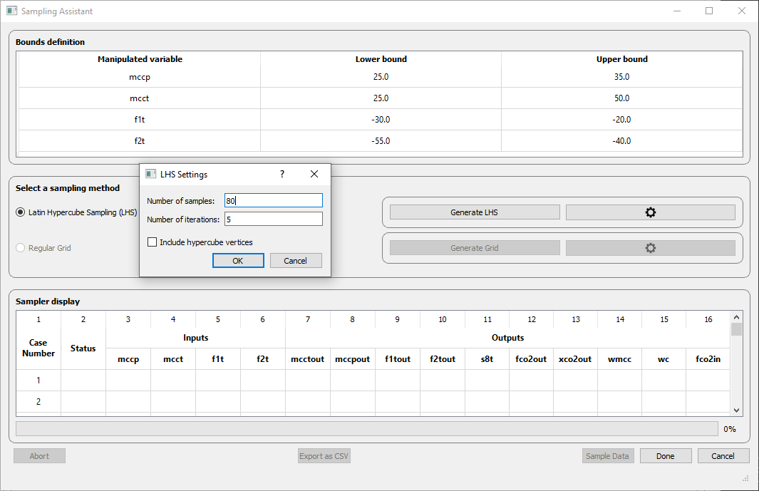
Fig. 100 Metacontrol Latin Hypercube Sampling settings. 80 samples were generated and 5 iterations were performed to maximize the minimum distance between the points (maxmin criterion). The user can also choose to add the vertices to the design.
After setting up the LHS, Metacontrol automatically runs each case in Aspen Plus via COM interface, communicating the results in the window showed in Fig. 101. After running all cases the user can then inspect the results of the design of experiments in a tabular form as depicted in Fig. 102.
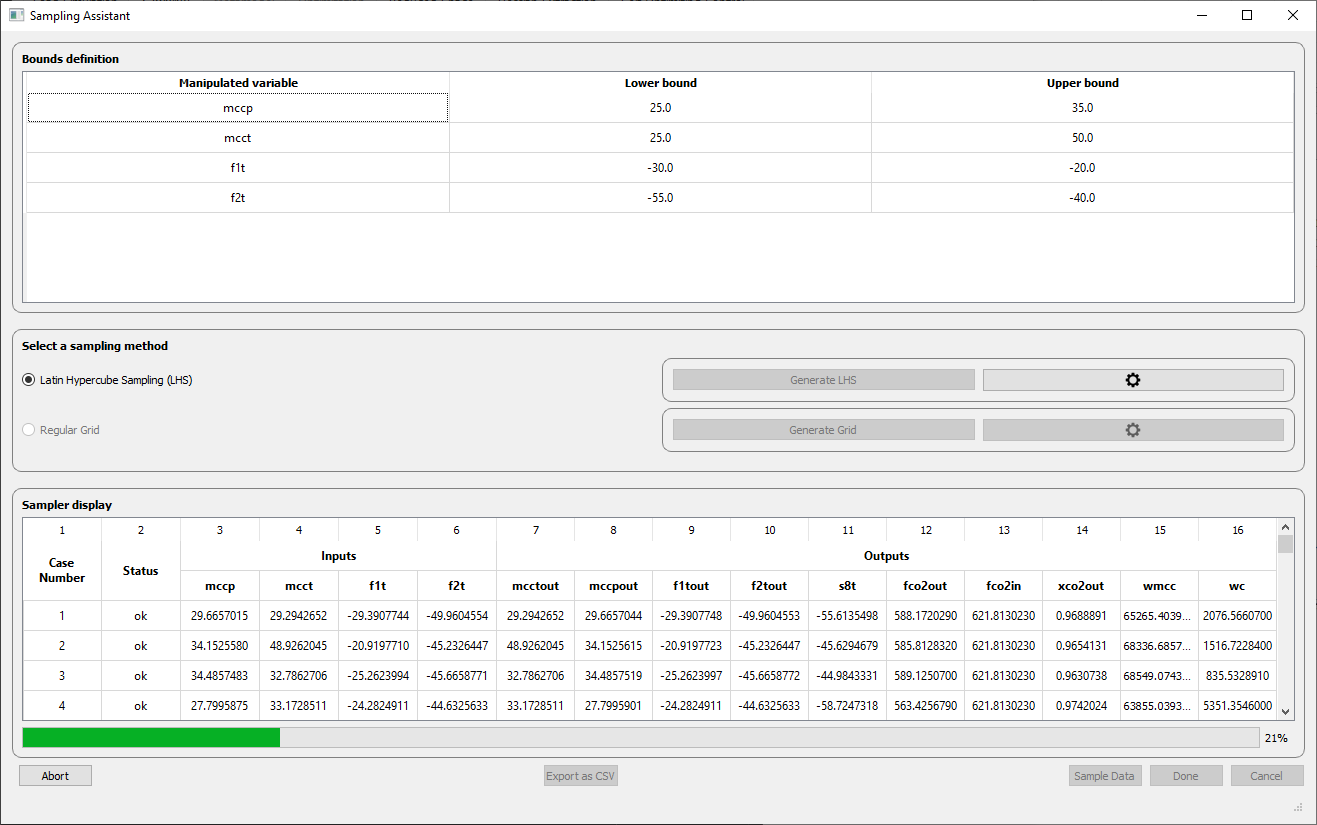
Fig. 101 Metacontrol Sampling for the \(CO_2\) CPU process.
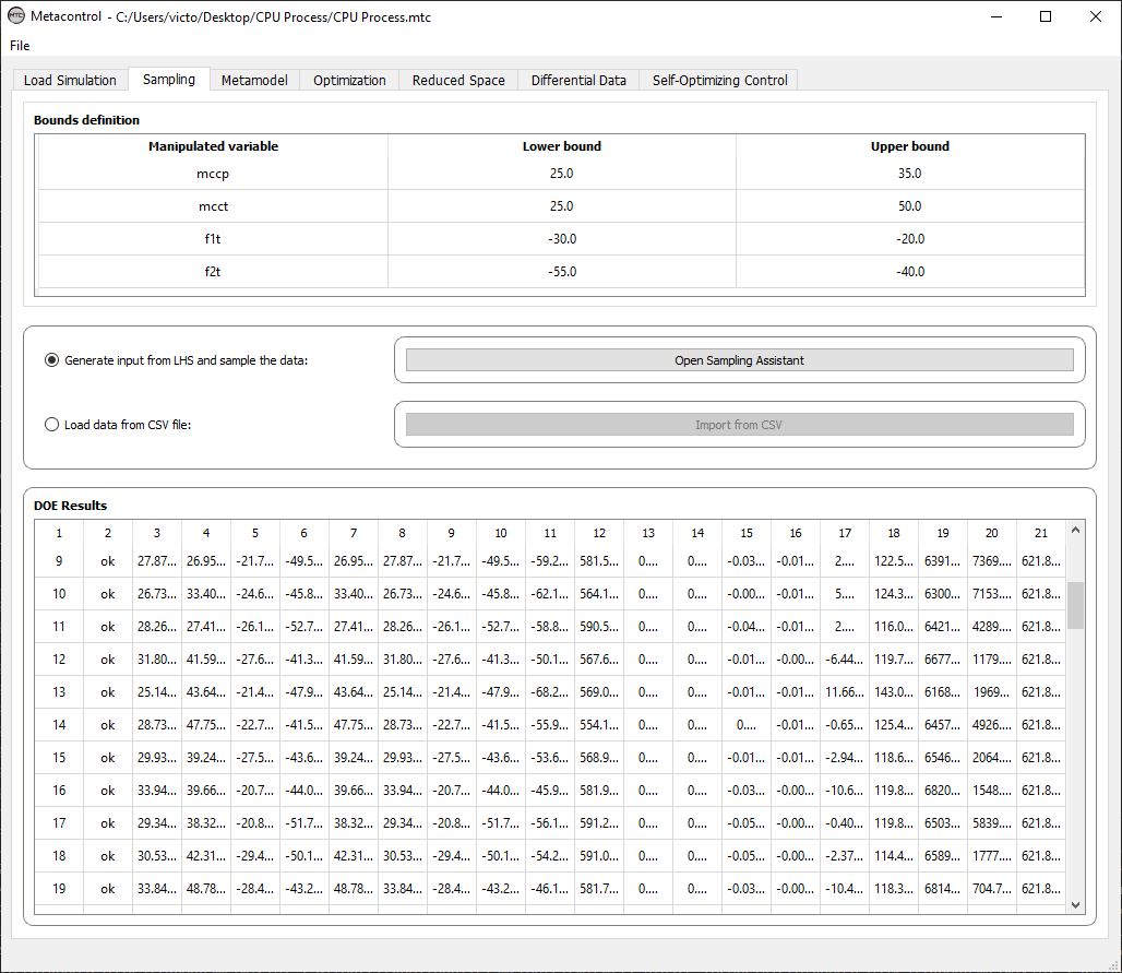
Fig. 102 Sampling results where the user can inspect convergence status and the values of the selected variables for each case.
Now the Kriging metamodel can be built. In the “Metamodel” Panel (Fig. 103) the user can select the response variables, define (initial) values for the bounds of the Kriging hyperparameters (\(\theta\)), choose regression and correlation models, and define the type of validation to be conducted. After hitting the button “Generate Metamodel”, the Kriging metamodel is generated, and if Hold-out is chosen as the validation mode it is possible to view the fitting results of each generated Kriging interpolator, as showed in Fig. 104. Moreover, good-of-fitness can be assessed by the available metrics Mean squared error (MSE), Root mean squared error (RMSE), Mean absolute error (MAE), \(R^{2}\) linear coefficient, Explained variance (EV), the Sample mean and also its standard deviation. It is important to point out that this first metamodel generation is performed only to allow for a quick view of the initial sampling, i.e., to check if the initial sampling is acceptable to be refined by the algorithm of [6] implemented in Metacontrol.
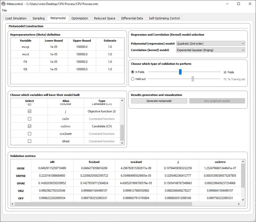
Fig. 103 Kriging configuration and validation metric results.
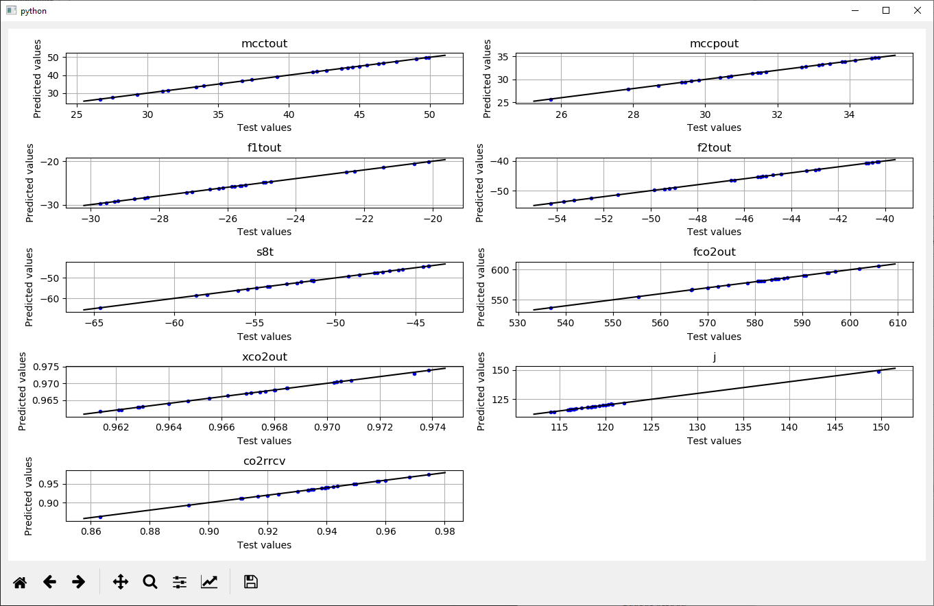
Fig. 104 Graphical validation for each metamodel.
The next step happens at the “Optimization” tab (Fig. 105) where advanced parameters of the algorithm of [6] and of the NLP solver can be tuned to improve the optimization of the Kriging interpolator. The final result of the refinement algorithm can be seen in the “Results” panel of Fig. 105 where the optimal values of the decision variables, constraint expressions, and the objective function are displayed. In addition, a log of the operations of contraction and movement of the hyperspace as the optimization progresses is showed.
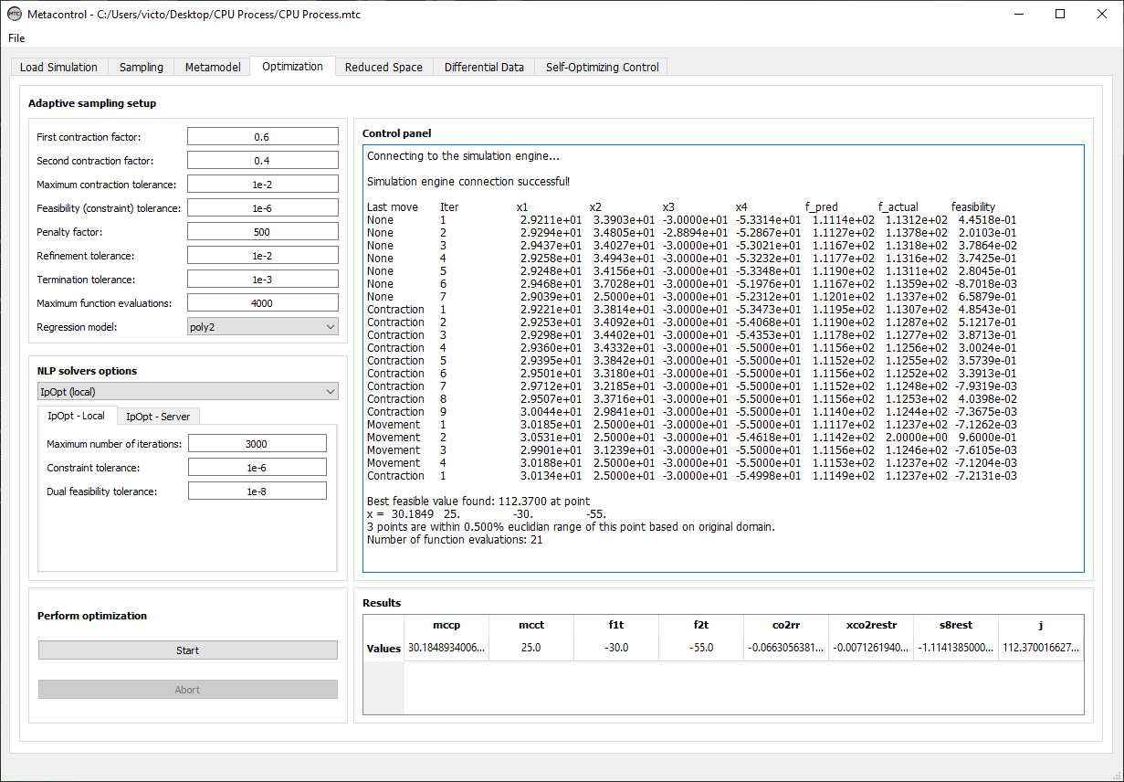
Fig. 105 Refinement algorithm configuration and results screen.
Table 5 and Table 6 shows the results of the optimization conducted at different conditions. Note there is almost no difference between the results of Metacontrol using the algorithm of [6] and Aspen Plus using the SQP algorithm, whereas for the optimization of the initial Kriging metamodel without refinement there is some discrepancy, as expected [11][20][6].
Objective function J (\(\frac{kW}{CO_2}\)) |
MCC Pressure (var) |
MCC Outlet Temperature (\(°C\)) |
F1 Temperature (\(°C\)) |
F2 Temperature (\(°C\)) |
|
|---|---|---|---|---|---|
Aspen Plus |
112.3690 |
30.0316 |
25.0 |
-30.0 |
-55.0 |
Metacontrol |
112.3691 |
30.1849 |
25.0 |
-30.0 |
-55.0 |
Initial Kriging |
113.5488 |
29.6672 |
34.8 |
-29.6 |
-52.3 |
Stream S8 temperature (\(°C\)) |
\(CO_2\) molar fraction |
\(CO_2\) recovery rate |
|
|---|---|---|---|
Aspen Plus |
-55.8201 |
0.9674 |
0.9658 |
Metacontrol |
-55.4859 |
0.9666 |
0.9671 |
Initial Kriging |
-56.0041 |
0.9685 |
0.9553 |
Three constraints were active at their lower bounds, namely the MCC outlet temperature and the temperatures of separators F1 and F2, and they need to be controlled for optimal operation (active constraint control). They are implemented in the simulation in Aspen Plus, e.g., either as input specifications or design specs, and then a Kriging metamodel representing the reduced space problem with only one degree of freedom left for self-optimizing control is generated either in a procedure similar to the generation of the initial Kriging metamodel or by importing a *.csv file with the results of the simulation runs. The latter might be considered when convergence is hard to achieve due to extra “feedback” loops caused by the implementation of active constraints in the process simulator or when the user feels more comfortable of running each case one at a time. In this case study, the *.csv import feature was showcased to illustrate its usage to the reader.
At the “Reduced space” tab (Fig. 106), on the “Variable activity” panel, the constraints that were active at the optimal solution must be marked together with the remaining independent variables not used to implement the active constraints in the process simulator (i.e., the unconstrained degrees of freedom). Also the values for the nominal disturbances must be specified. When sampling the reduced space problem using the process simulator via Metacontrol, the range of the remaining decision variables and disturbances must also be defined. It goes without saying that this range should be as small as possible (around \(\pm 0.5\%\) of the nominal optimum) to produce a surrogate model accurate enough at the optimal region in order to guarantee robust gradients and Hessians [3].
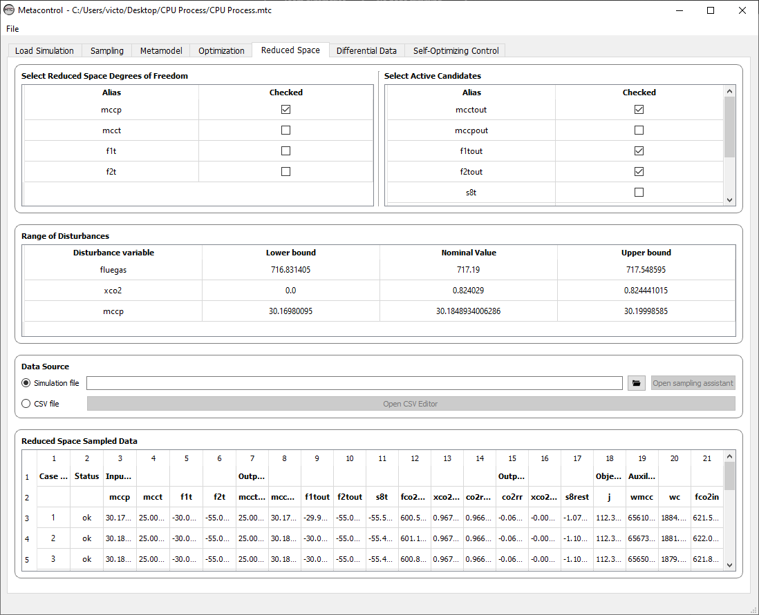
Fig. 106 “Reduced space” tab to define the reduced space model requirements.
A *.csv file containing the results of a sensitivity analysis conducted in the process simulator under active constraint control was loaded in Metacontrol, as illustrated in Fig. 107. Note that the denominations of the variables in the *.csv file must be associated to the respective variables in Metacontrol.
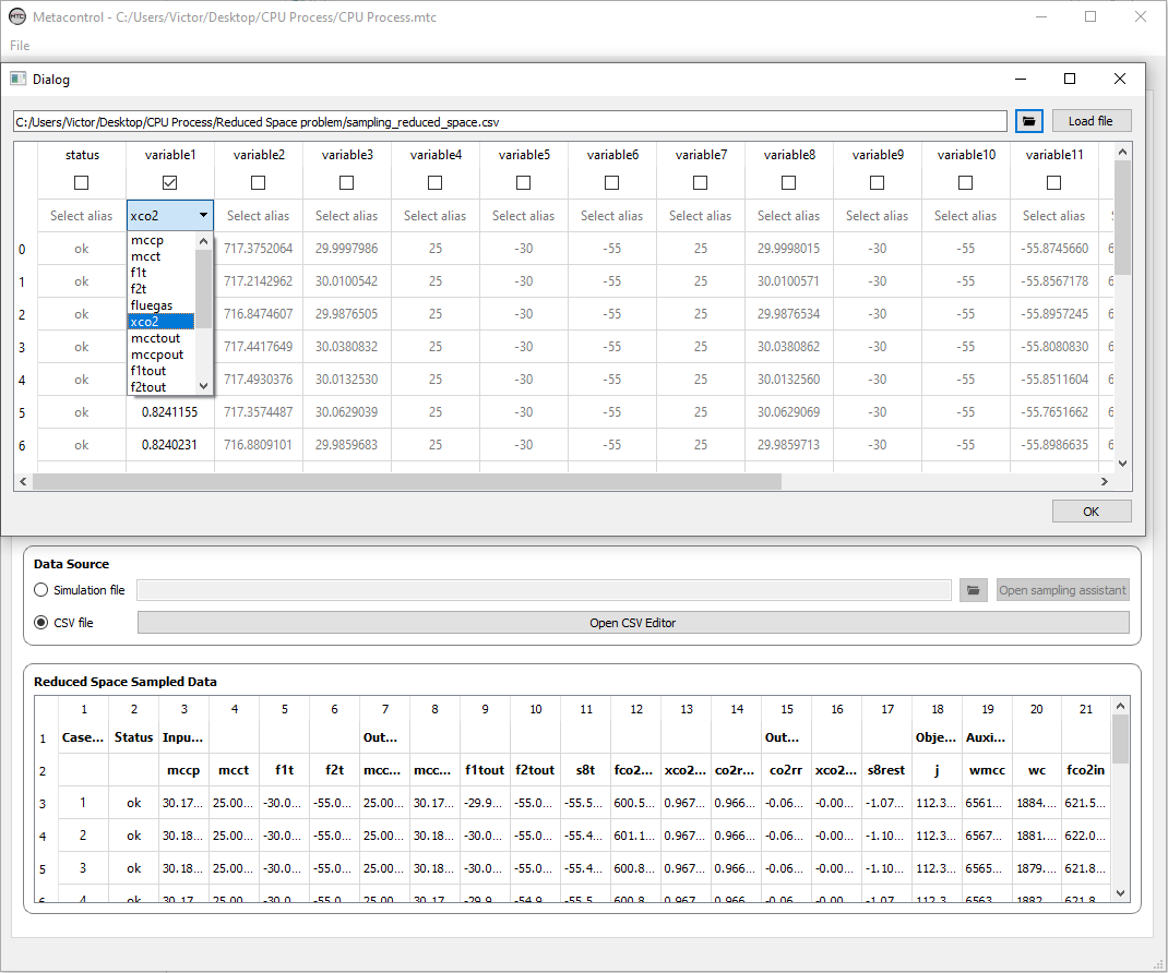
Fig. 107 Associating each alias created in Metacontrol to each column of the *.csv data.
Now that the data is available, the reduced space Kriging metamodel can be generated. Under the panel “Reduced space metamodel training” on the “Differential data” tab (black rectangle in Fig. 109), hitting the button “Open training dialog” allows for the tuning of the Kriging parameters and metamodel construction (Fig. 108).
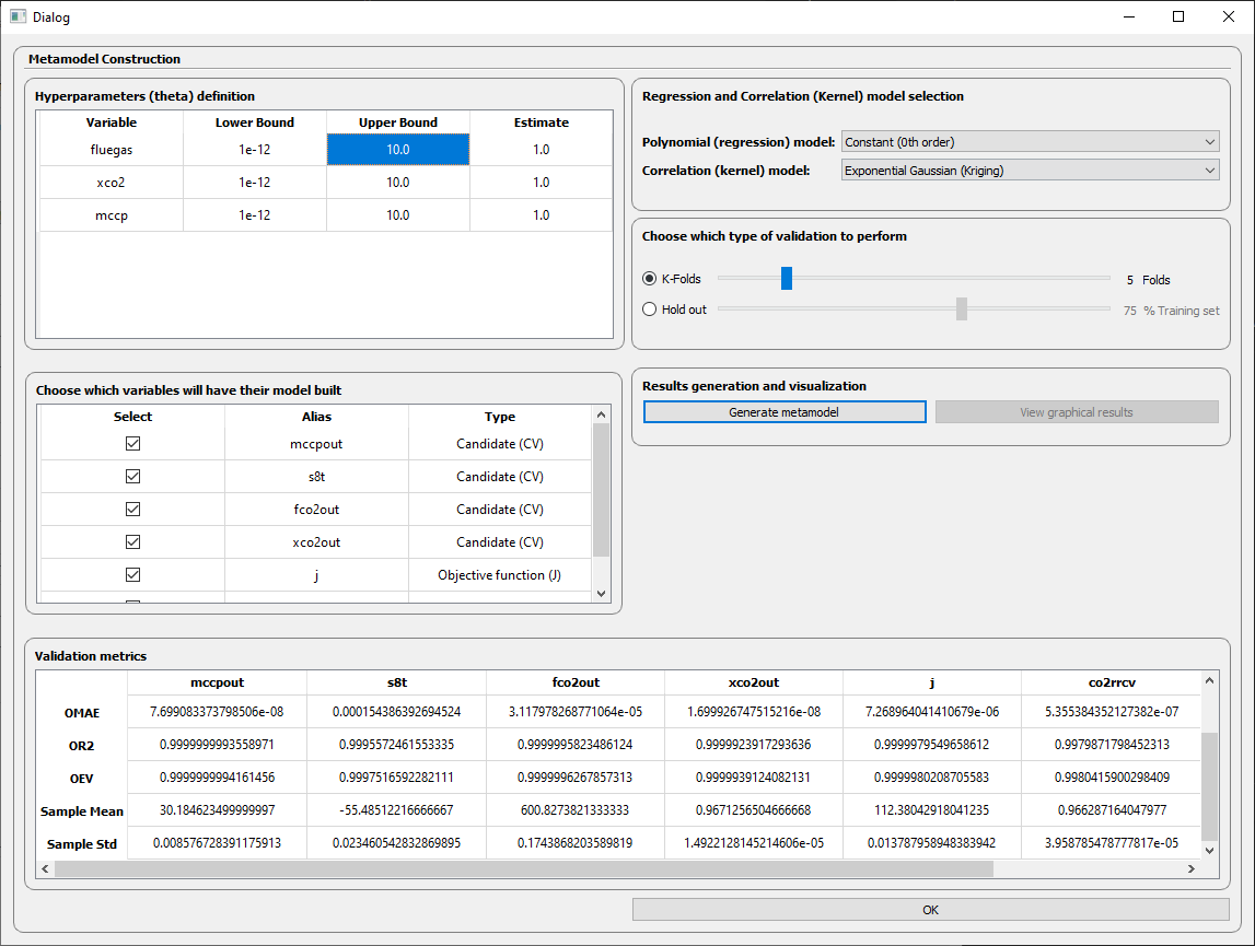
Fig. 108 Generating the reduced space metamodel for the \(CO_2\) CPU process.
Heading back to the previous screen (Fig. 109), gradients and Hessians necessary to carry on the Self-Optimizing control analysis can be computed via analytical expressions of the these derivatives as developed by [26] and [3]. For this case, the gradients calculated in Metacontrol agree with those provided by Aspen Plus under the Equation Oriented mode, as shown in Table 7 (note the mean-squared errors are very small).
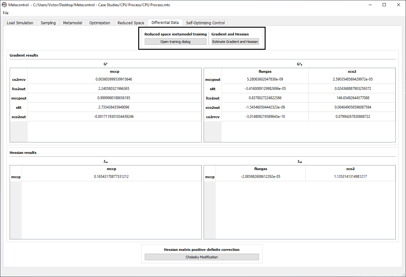
Fig. 109 Computation of derivatives in Metacontrol.
\(G^{y}\) |
\(G_{d}^y\) |
|
|---|---|---|
Metacontrol |
\(\begin{bmatrix} 0.00360399953991565\\ 2.24058032196637\\ 0.999998018865619\\ 2.73543843594910\\ -0.00171193010344392 \end{bmatrix}\) |
\(\begin{bmatrix} -3.01480921958964e-10 & 0.0799426783086872\\ 0.837802722482259 & 146.654926445771\\ 5.28063602047838e-09 & 2.59035485694300e-05\\ -3.41600891299827e-05 & 0.0243688879032594\\ -1.54546050444232e-09 & 0.00404905859608759 \end{bmatrix}\) |
Aspen Plus |
\(\begin{bmatrix} 0.00360289000000000\\ 2.24032100000000\\ 1\\ 2.73303800000000\\ -0.00171230000000000 \end{bmatrix}\) |
\(\begin{bmatrix} 1.34722000000000e-07 & 0.0798491000000000\\ 0.837799400000000 & 146.612400000000\\ 0 & 0 \\ 3.37970000000000e-15 & 0.0249510000000000\\ 1.69120000000000e-16 & 0.00404464000000000 \end{bmatrix}\) |
Mean-squared error |
1.16586918414966e-06 |
1.8088e-04 |
As a requirement of the procedure, the magnitude of disturbances and measurement errors can be specified in the “Self-Optimizing Control” tab ( Fig. 110). For the \(CO_{2}\) inlet composition this magnitude was \(0.05\) and for the flue gas flow rate it was considered \(5\%\) of the nominal optimum value. The measurement errors were set to \(0.5°C\) for temperatures, \(0.01\) for pressures and flow rates, and \(0.001\) for ratios (\(CO_{2}\) recovery rate and product purity). The number of best subsets of a given size to be evaluated as possible candidates was specified under the “Subsets sizing options” panel. By clicking on the “Generate results” button a dialog window shows the results of the self-optimizing control calculations.
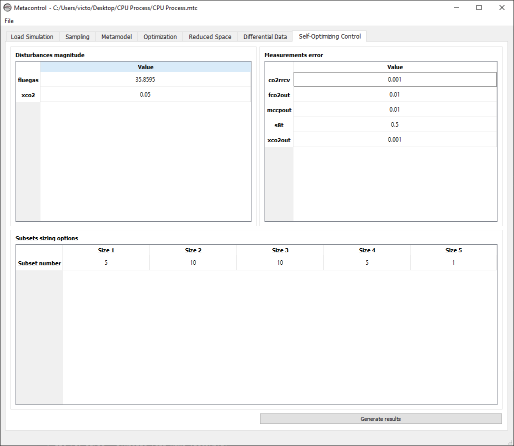
Fig. 110 Defining parameters for self-optimizing computations.
Fig. 111 and Fig. 112 detail the results for the single measurement policy (subset size 1) and for the configuration using a linear combinations of 2 measurements (subset size 2), respectively. Also depicted are the \(H\) matrix and the optimal sensitivity matrix \(F\) for each subset.
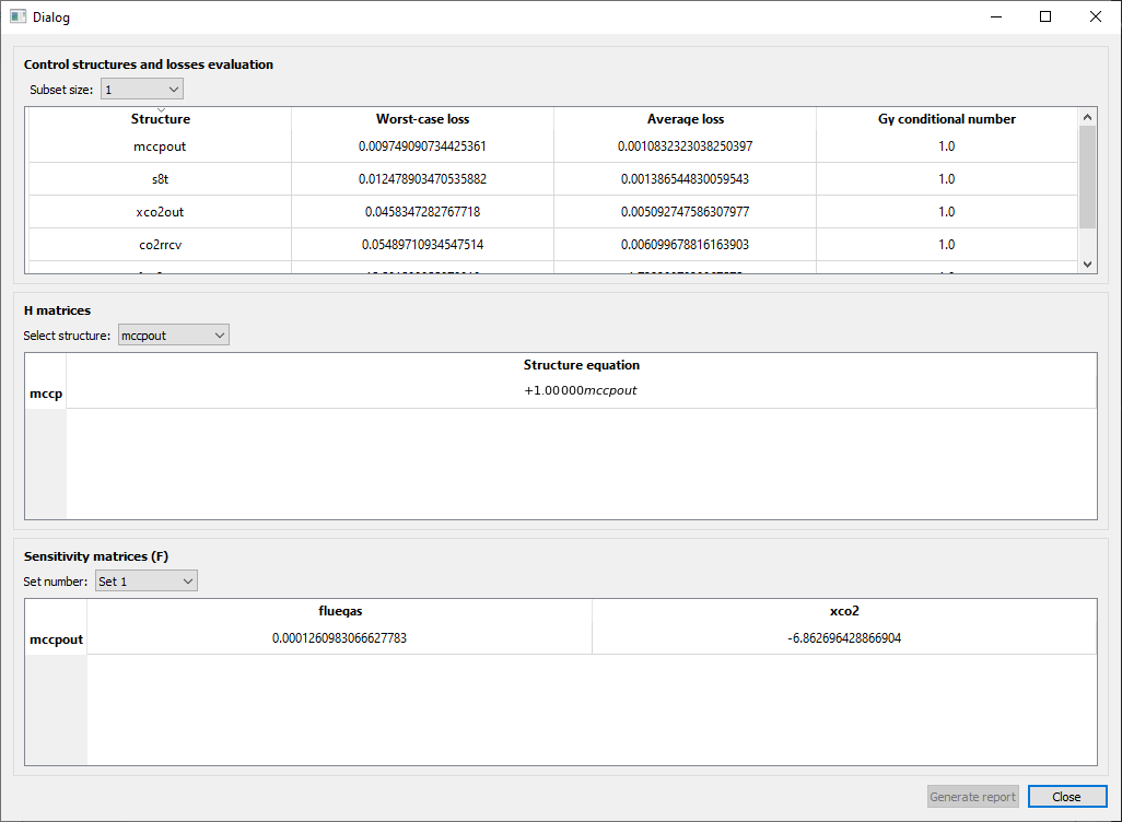
Fig. 111 Best selected controlled variables for the single measurement policy.
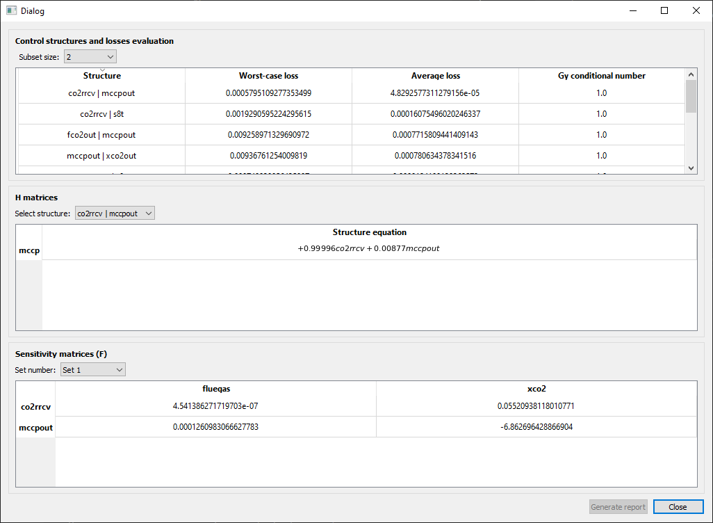
Fig. 112 Best selected controlled variables for linear combinations of 2 measurements.
Table 8 is a summary of the results for the single measurement policy showing that controlling the multi-stage compressor (MCC) outlet pressure at its nominal optimal value leads to (near) optimal operation, despite of disturbances and measurement errors. This result compares to the previous findings of [24], where similar control structures were proposed. However, they heuristically assumed control of process constraints in contrast to the SOC procedure used in Metacontrol.
Candidate controlled |
Worst-Case |
Average-Case |
variable |
Loss \((kWh/tCO_{2})\) |
Loss \((kWh/tCO_{2})\) |
mccpout |
0.009749090734425361 |
0.0010832323038250397 |
s8t |
0.012478903470535882 |
0.001386544830059543 |
xco2out |
0.0458347282767718 |
0.005092747586307977 |
co2rrcv |
0.05489710934547514 |
0.006099678816163903 |
fco2out |
15.591598055970818 |
1.7323997839967575 |
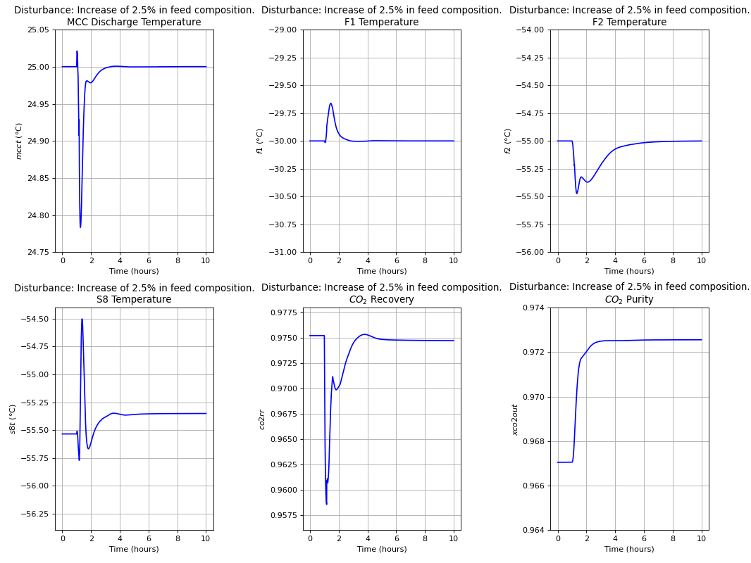
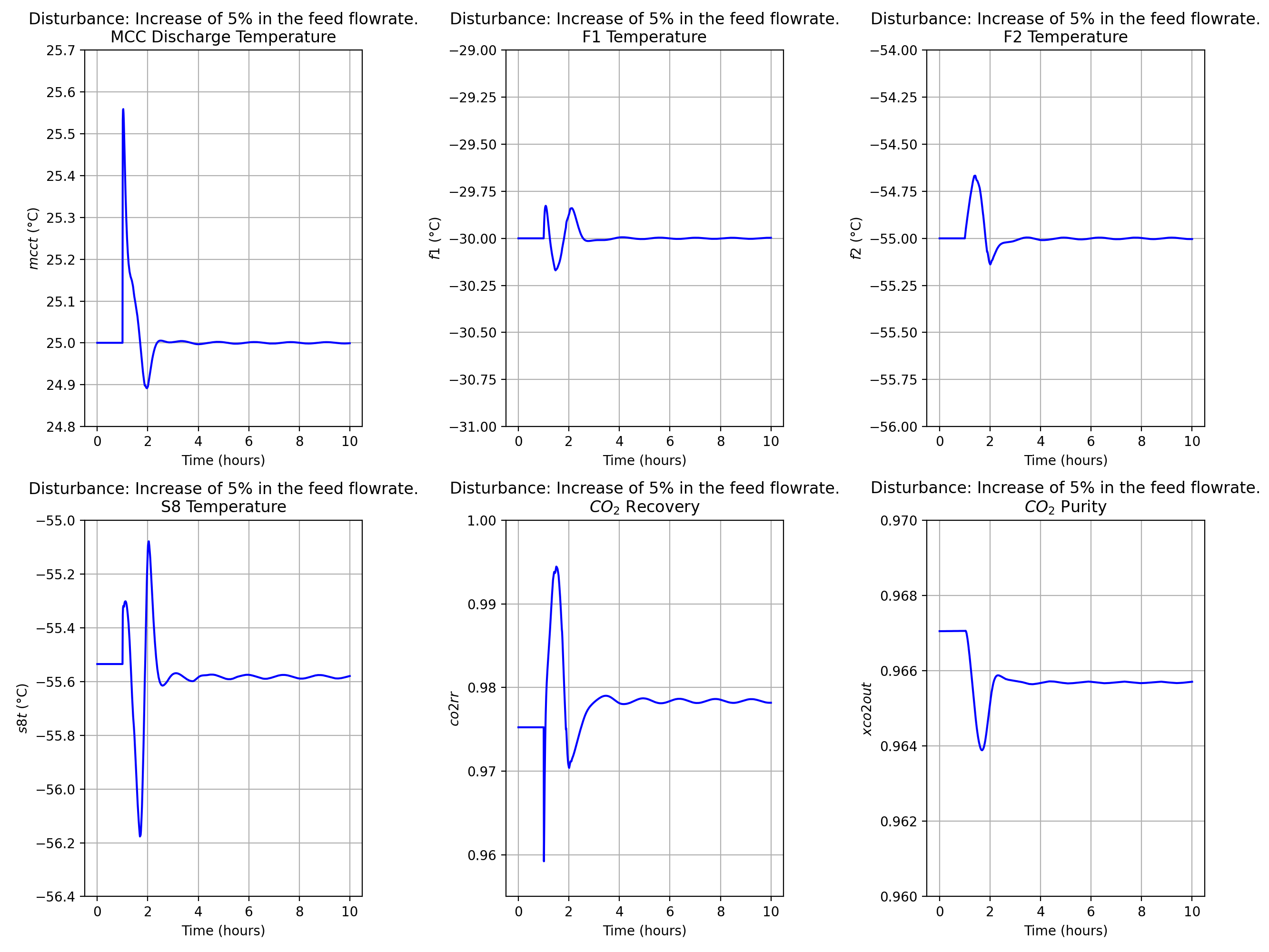
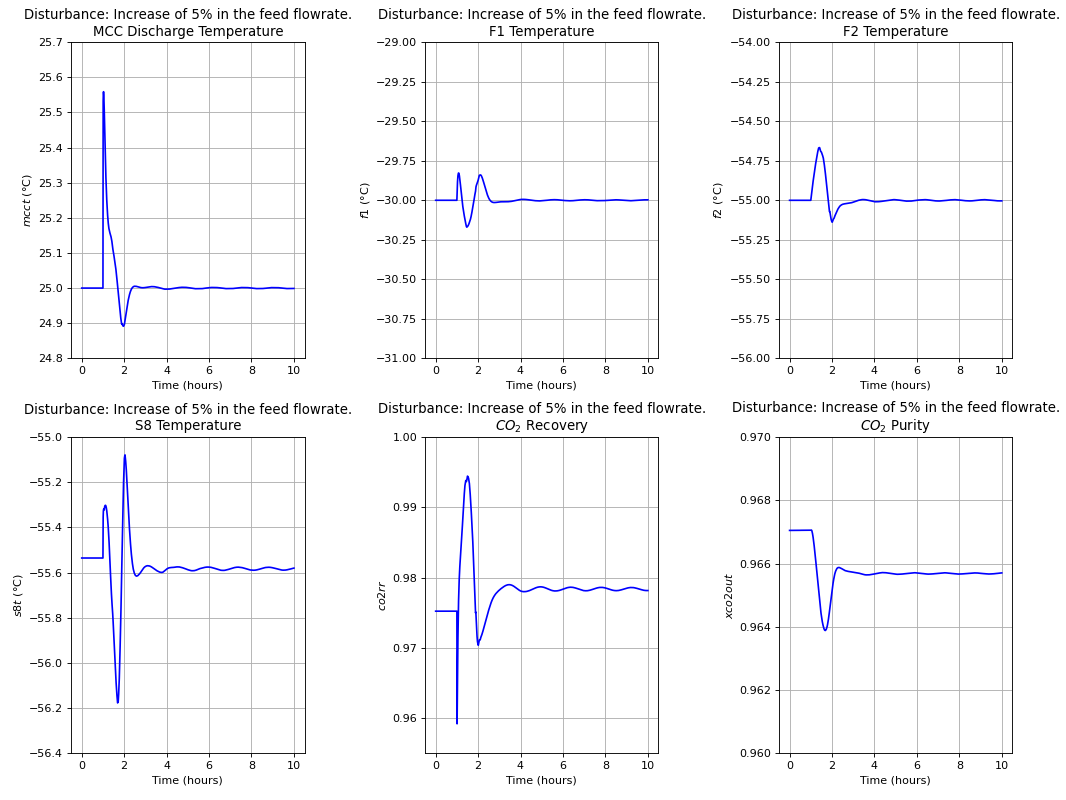
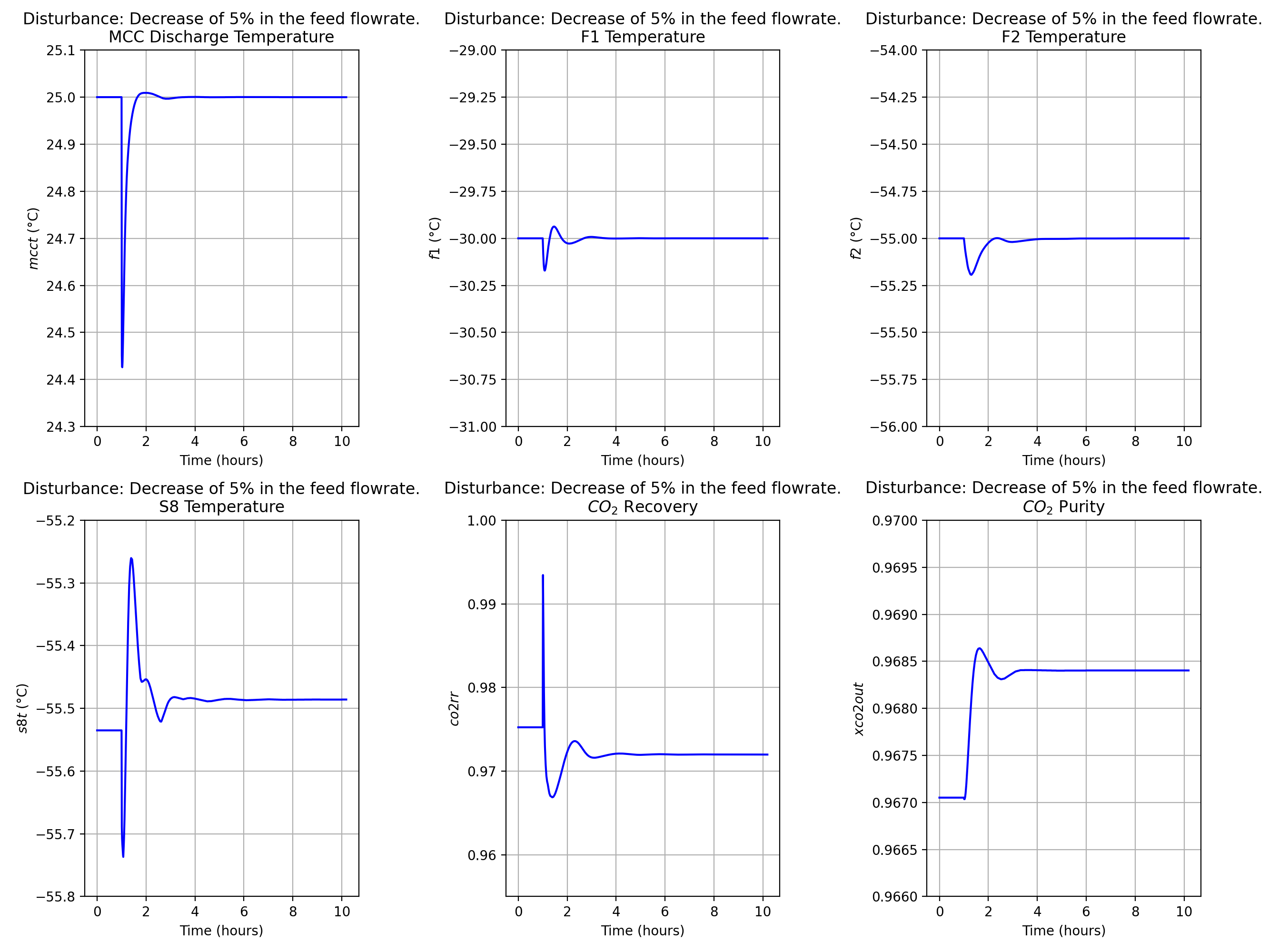
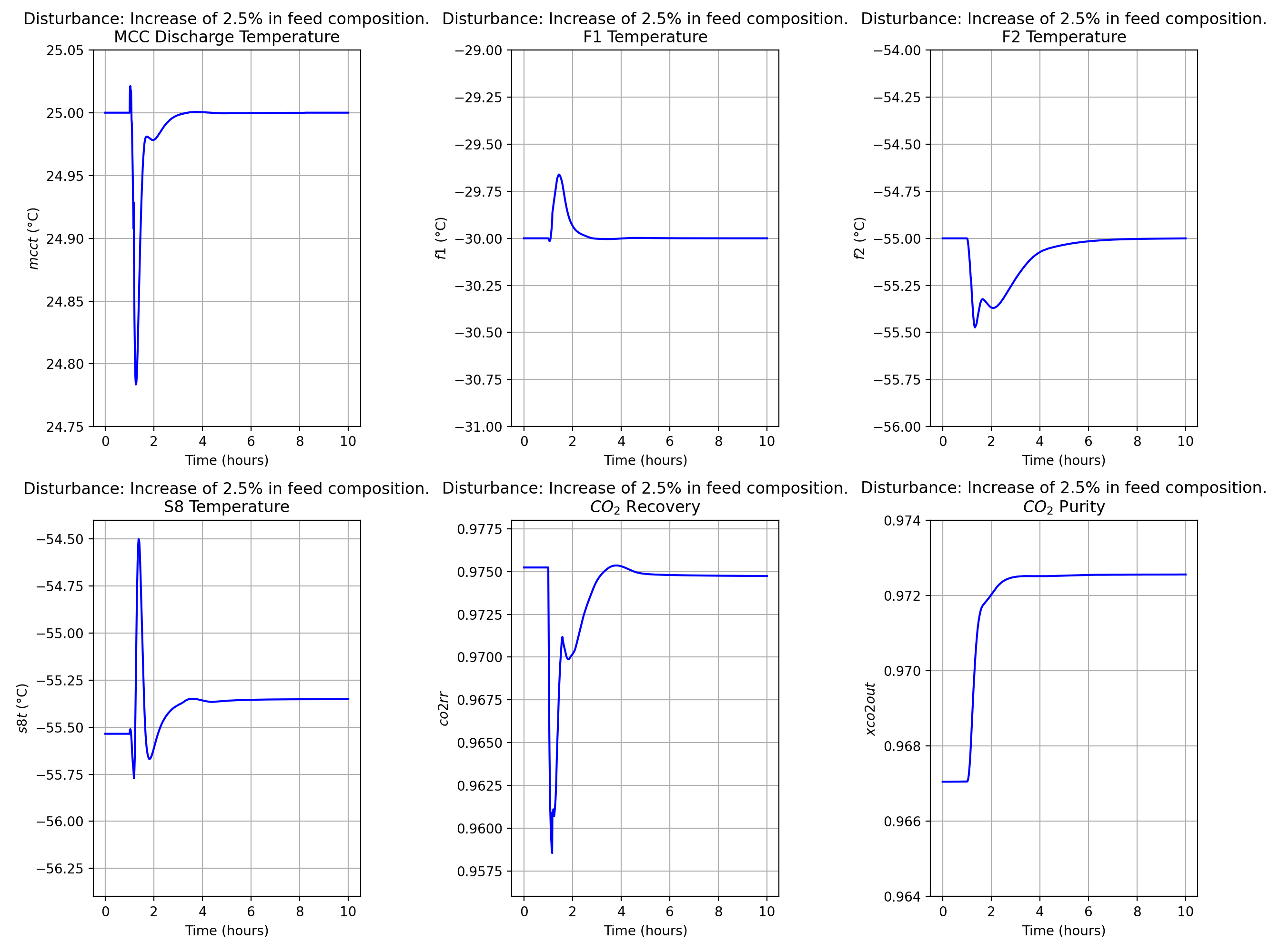
Dynamic simulations
The dynamic evaluation of the control structure using the S-8 Stream temperature as the unconstrained controlled variable was performed according to the Single Temperature Control (STC) of [19]. Note that this choice of controlled variable was a consequence of the systematic procedure embedded in Metacontrol, and not an heuristic-based decision. Control of the MCC discharge pressure, though incurring in the lowest economic loss, was not considered on the basis of large flow rate fluctuations that can eventually come from the boiler island to upset the CPU Process. The following plots show the result of dynamic simulations where it can be seen the robust performance of the proposed SOC-Based control configuration. It is worth mention that the constraint regarding stream S-8 lowest temperature due to \(CO_{2}\) freezing point was not violated. Simple PI controllers were used, with IMC tuning rules and a process flowsheet depicting the control configuration in place is provided in Fig. 113.

Fig. 113 Control structure tested.
