The “Reduced Space” tab
At this tab you will define your Reduced-Space problem:
Generate the reduced space problem DOE data, in order to generate a kriging metamodel around the nominal optimal operating point found in the previous step. The idea here is to generate a metamodel with points sampled around a small deviation from the optimal point, to generate the gradients with respect to the plant measurements, to the disturbances, and the hessians, with robustness, as proved by ([3]).
Additionally, you will inform Metacontrol which constraints are active, and what are the remaining degrees of freedom that are going to be used at the Reduced Space problem sampling, at the “Variable activity” panel.
Inform the bounds of the Manipulated variables and disturbances around the optimal point.
Here is an overview of this tab:
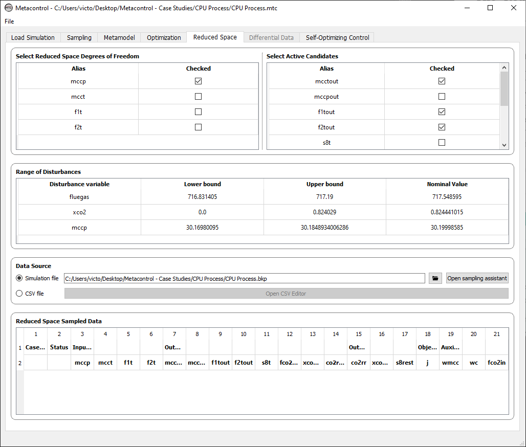
Fig. 48 Metacontrol “Optimization” tab.
There are four main panels at this tab:
Variable activity panel
Range of Reduced-space Variables panel
Data source panel
Reduced Space sampled Data panel
Important
At this point, you must go back to the process simulator (Aspen Plus), and implement the active constraints that were found by the optimization step.
Save a copy of your initial .bkp file.
In your copied simulation file, implement your active constraints:
If they are input specifications, just fix their values at the respective block or stream where the variable is located.
If they are output variables, implement Design Specifications, consuming the necessary degrees of freedom.
Save and close your Reduced-Space problem aspen plus file.
Go back to Metacontrol.
Variable activity panel
At this panel, you will inform to Metacontrol the reduced-space remaining degrees of freedom (e.g.: The variables that were not used to close feedback loops in case of nonlinear constraints becoming active, or the the decision variables that did not reached an upper/lower bound at the optmization run). Metacontrol automatically understands that the variables that you did not check, were active decision variables or were used as MVs for a desing specification loop. On the right panel, you should indicate if any CV candidate that you created (which eventually can be a constraint) were active. You should mark these variables, since you must control them (Active-Constraint Control [31]), before using the mathematical formulations that are implemented within Metacontrol.
Informing to Metaconrol active candidates and active decision variables (MVs)
At example in the figure below, mcct, f1t and f2t were nominally active at the optimal point. These are the Manipulated Variables of this example. The remaining variable corresponds to mccp. Therefore, at the left side of the “Variable activity” panel, only the remaining degree of freedom must be checked (mccp):
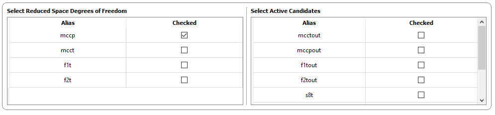
Fig. 49 Selecting unconstrained degree(s) of freedom.
On the other hand, the variables mcctout, f1out and f2out are the decision variables (MVs) also listed as CV candidates, in order to analyze if keeping them constant, there will be self-optimizing control structures using them. Since the decision variables were active, they must be eliminated from the list of potential candidates, since the SOC methodology considers that active-constraint control is a mandatory step of the methodology. Therefore, you must mark them as active:
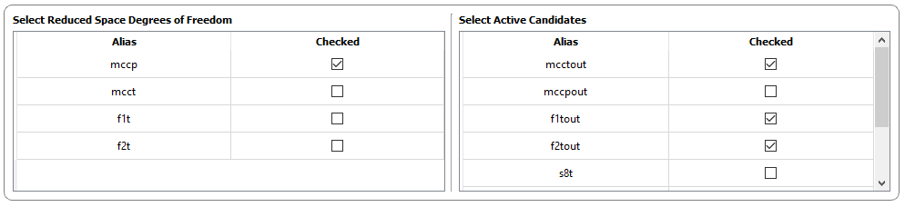
Fig. 50 Selecting unconstrained degree(s) of freedom.
Important
In a nutshell, this panel serves for you to inform to Metacontrol what are the unconstrained degrees of freedom of the reduced-space problem, and also to inform the active candidate controlled variables (constraints, MVs listed as candidates, etc.). With this information, Metacontrol will automatically consider only the unconstrained degrees of freedom summed with the disturbances as input variables on the sampling, and also will not consider the active variables when generating the high-order data (gradients and hessians). Since you are providing a modified simulation file with the active variables implemented (MVs and or constraints/CVs), they do not need to be in the analysis, since they are already being controlled.
Range of Reduced-space Variables panel
On this panel, you will inform the lower and upper bound of the unconstrained degrees of freedom and disturbances to be used in the sampling process, in order to generate the reduced-space kriging metamodel:
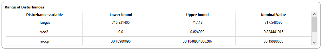
Fig. 51 Selecting unconstrained degree(s) of freedom.
Important
As showed on our previous publications, the bounds for the second (reduced-space) kriging metamodel must be a around a small margin of the optimal operating point. You can consider this a tunable parameter. Generally, +-0.5% of the optimal operating point will generate robust prediction of the high-order data on the next step (gradients and hessians). However, feel free to tight or loose this value if you want to try to improve your reduced-space kriging metamodel.
Data Source panel
On this panel you will:
Point to the Aspen Plus simulation file of the reduced-space problem, if you opt to sample using the process simulator.
Use the sampling assistant, if you opt to sample using the process simulator.
Point to the .csv file if you opt to import an already sampled DOE of the reduced space problem.
Sampling the reduced-space problem with your Aspen Plus simulation file
Under the Data Source panel, point to the Aspen Plus reduced-space problem file location:
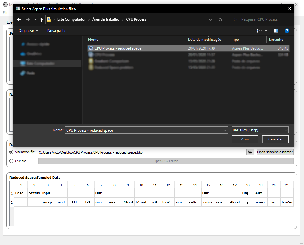
Fig. 52 Pointing to the reduced-space problem simulation file.
After this, you can open the Sampling Assistant:
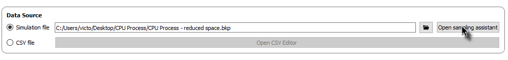
Fig. 53 Opening the sampling assistant.
You will notice that the Sampling Assistant window corresponds exactly to the same from the step 2 (Using the Sampling Assistant to sample data from Aspen Plus). Therefore, the procedure is exactly the same.
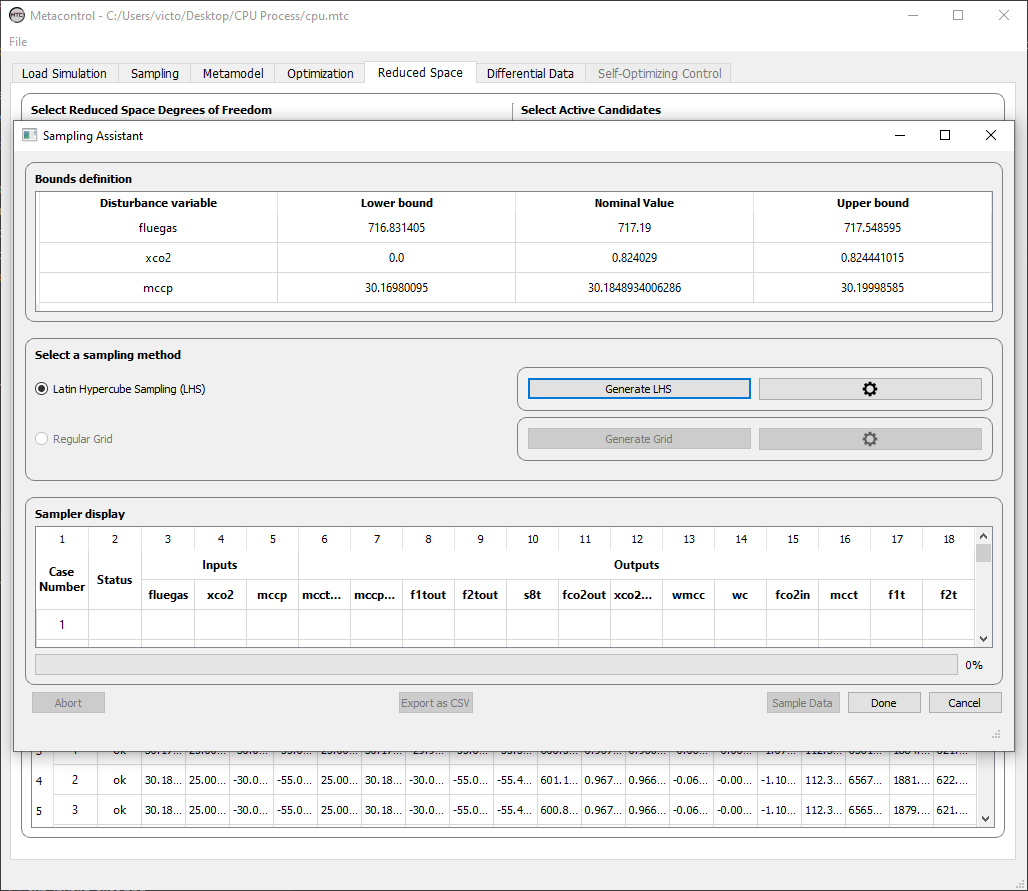
Fig. 54 The sampling assistant, the same from the sampling tab.
You will define the number of cases to be sampled:
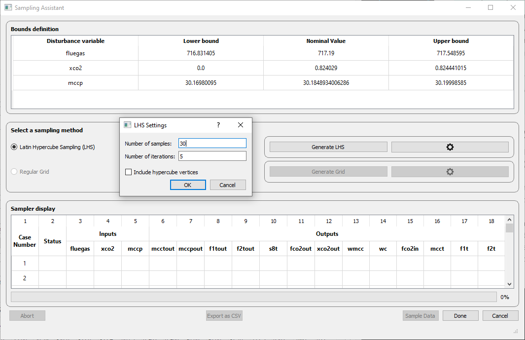
Fig. 55 Configuring the number of cases to be sampled.
And click on “Sample Data”. You can at any time, abort this operation (“Abort” button). When the sampling is finished, you can click on “Done” and proceed to the next step (Differential data).
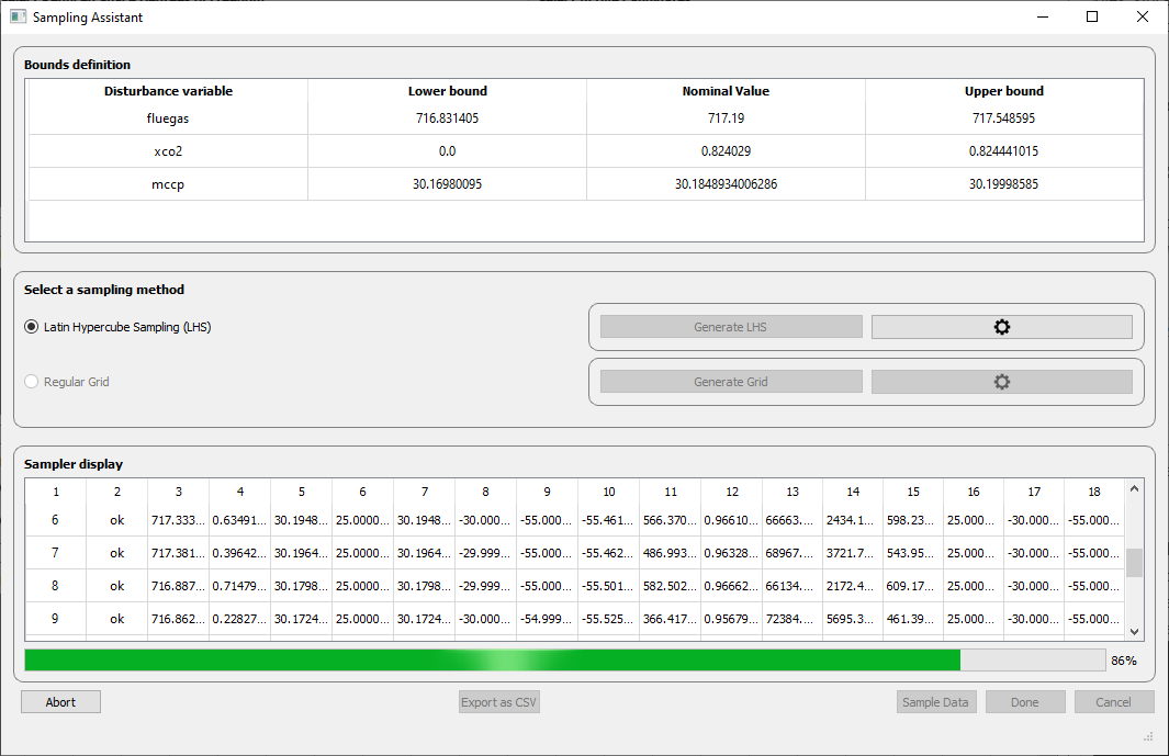
Fig. 56 Sampling Assistant running cases for the reduced space problem.
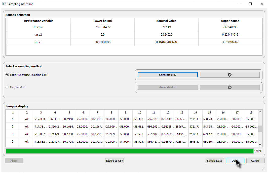
Fig. 57 Sampling completed, just click on “Done” to go back to “Reduced Space” tab.
Reduced Space sampled Data panel
After sampling you data, if you go back to the Reduced Space Tab, you will notice that this panel will be completed:
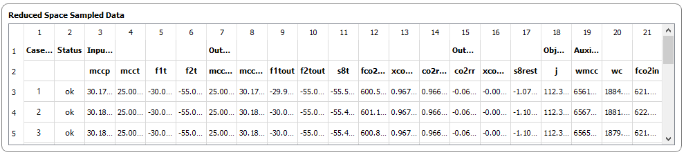
Fig. 58 Reduced Space sampled Data panel.
After everything, your Reduced Space tab will be completed:
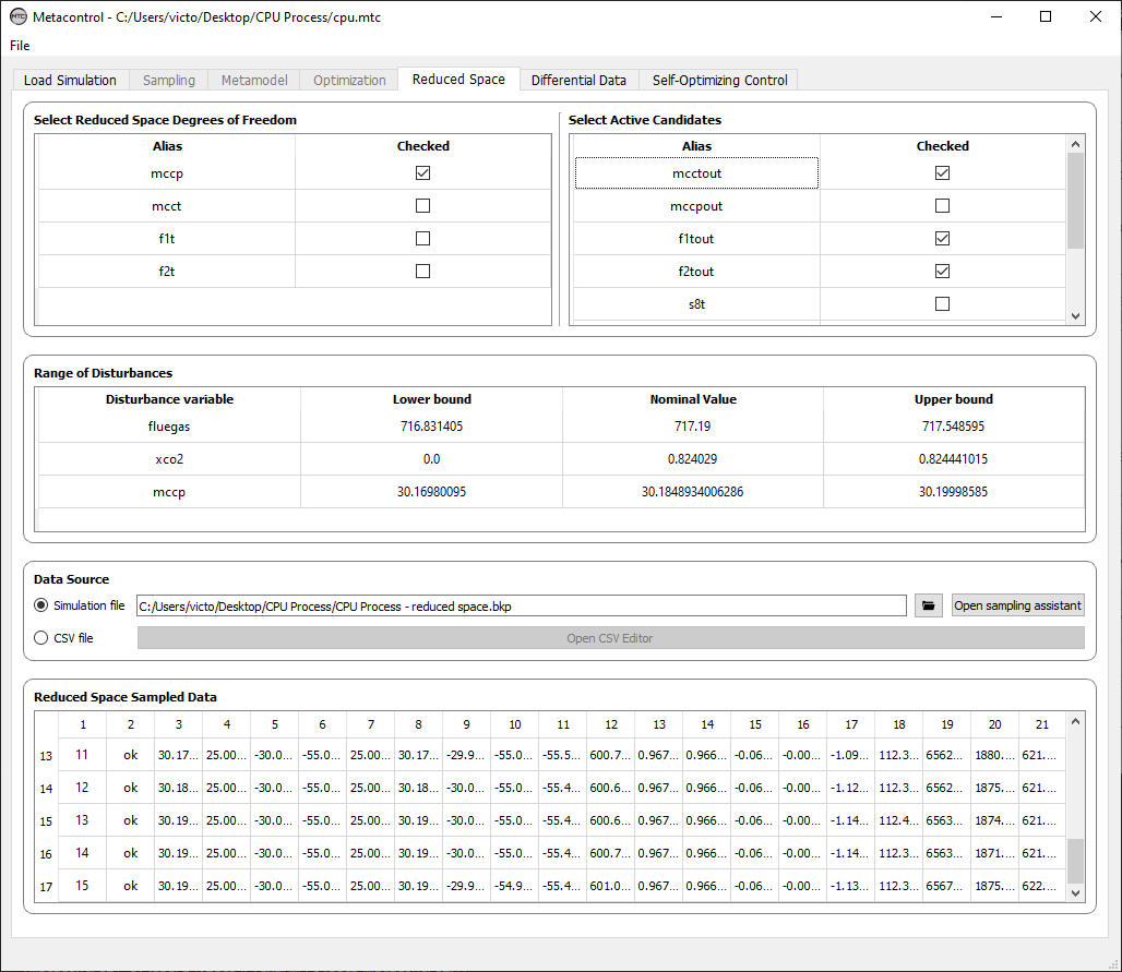
Fig. 59 Reduced space tab completed. You are able to go to the next tab (Differential data).