The “Sampling” tab

At this tab you will use the simulation provided on the previous step to perform a Design of Experiments (DOE). You will be able to:

• Define the lower and upper bounds for your manipulated variables, that will be used as the limits of the sampling and as box constraints of the optimization problem

• Define the number of sampled cases

• Inspect the results of the sampling, for each variable that you selected on the previous step

• Check convergence status of each case

Here is an overview of this tab:

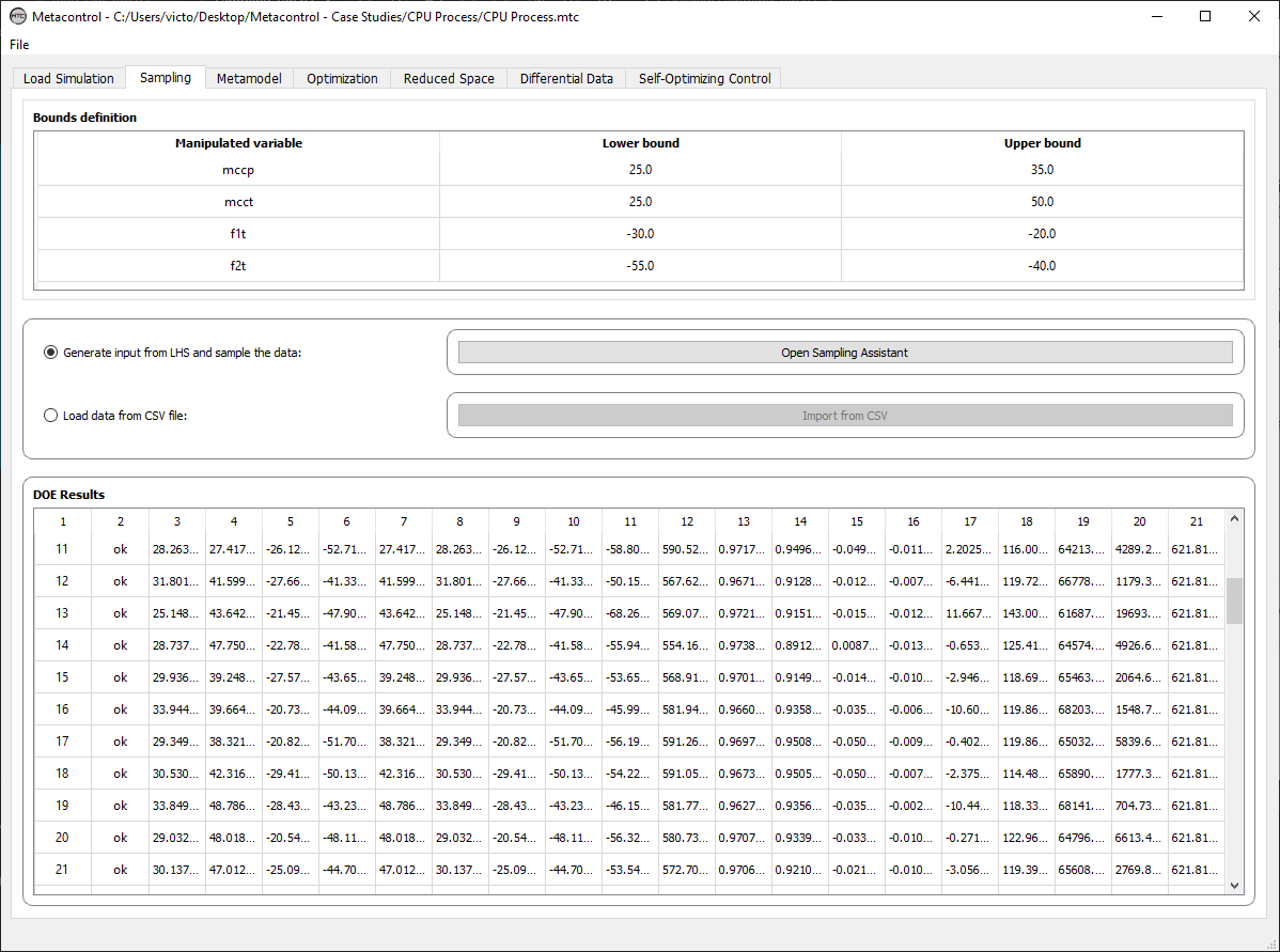
Fig. 19 Metacontrol “Sampling” tab.

There are three main panels on this tab:

• Bounds definition panel

• Sampling assistant panel

• DOE Results panel

Bounds definition panel

This is the panel that you will define the upper and lower bounds of the Manipulated Variables that you chose. These limits will be used to sample your data, if you choose to use your Aspen Plus model in order to do so. In addition, these limits will be automatically used as box constraints at the optimization step. Note that the aliases that you chose for you Manipulated Variables are neatly shown here.

Fig. 20 Bounds definition panel.

Inserting the lower and upper bounds for your MVs

That’s pretty straightforward. Simply click on each variable “Lower Bound” and “Upper Bound” field, and type it:

Fig. 21 Insert bounds for your MVs.

Sampling Assistant panel

This panel defines how are you going to supply the DOE data to metacontrol: Using your simulation file (recommended) or loading an .CSV file (this is an auxiliary feature). For the first case, you are going to use the Sample Assistant from *Metacontrol:

Using the Sampling Assistant to sample data from Aspen Plus

Click on “Open Sampling Assistant”:

Fig. 22 Selecting the Sampling Assistant.

The Sampling Assistant Screen will be revealed:

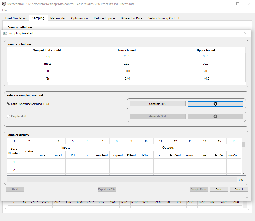
Fig. 23 Selecting the Sampling Assistant.

Important

Currently, Latin Hypercube Sampling (LHS) is the main sampling technique used in Metacontrol. Check our publications for a justification for its usage.

Clicking on the “Gear” Icon at the “Select a Sampling Method” panel, you will be able to define the number of desired cases and how many iterations the LHS routine will perform in order to improve the sampling. Generally, a value of 5 is enough. In this case, we are going to run 80 cases. In addition, you can opt to include the vertices of the hypercube of your design.

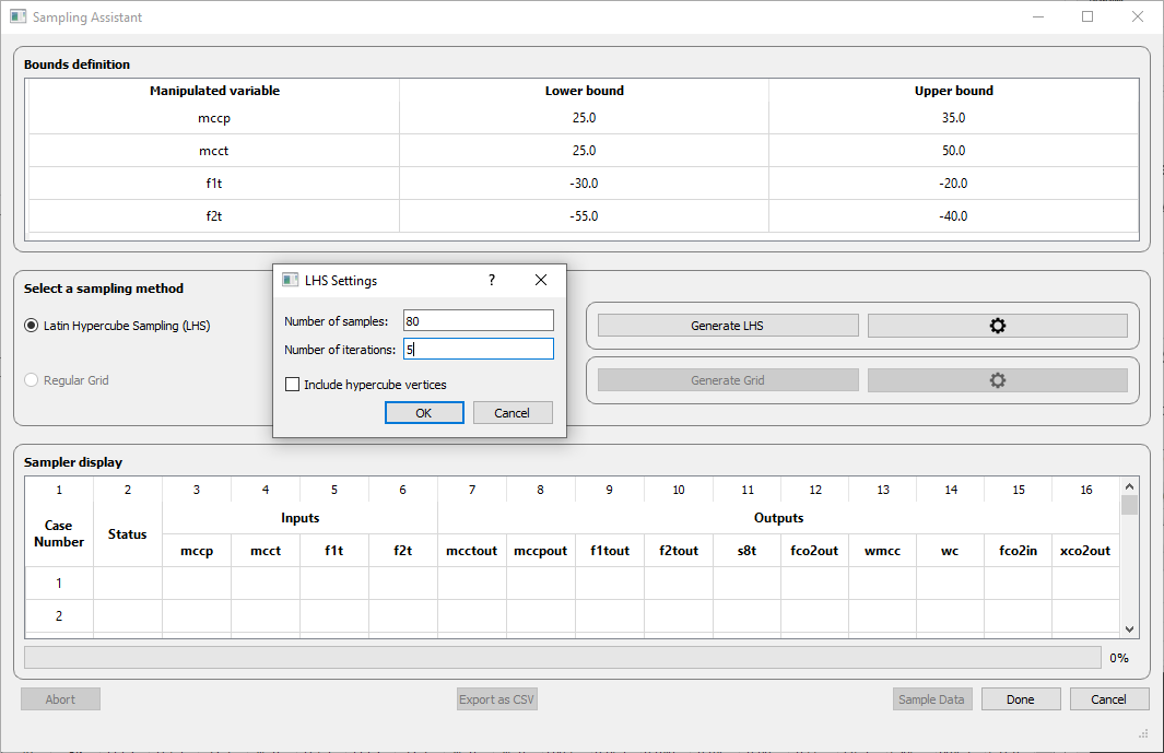
Fig. 24 Defining the number of cases.

Clicking on “ok” will bring you to the previous screen, and you can generate the input data by the LHS method:

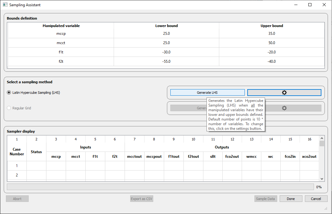
Fig. 25 Generating LHS Input data.

Notice that now under the “Sampler Display” panel, the LHS Input data is show (Here, intentionally highlighted in blue):

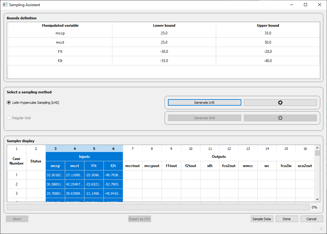
Fig. 26 LHS Input data.

The “Sample Data” button now is available. Push it to start running your cases.

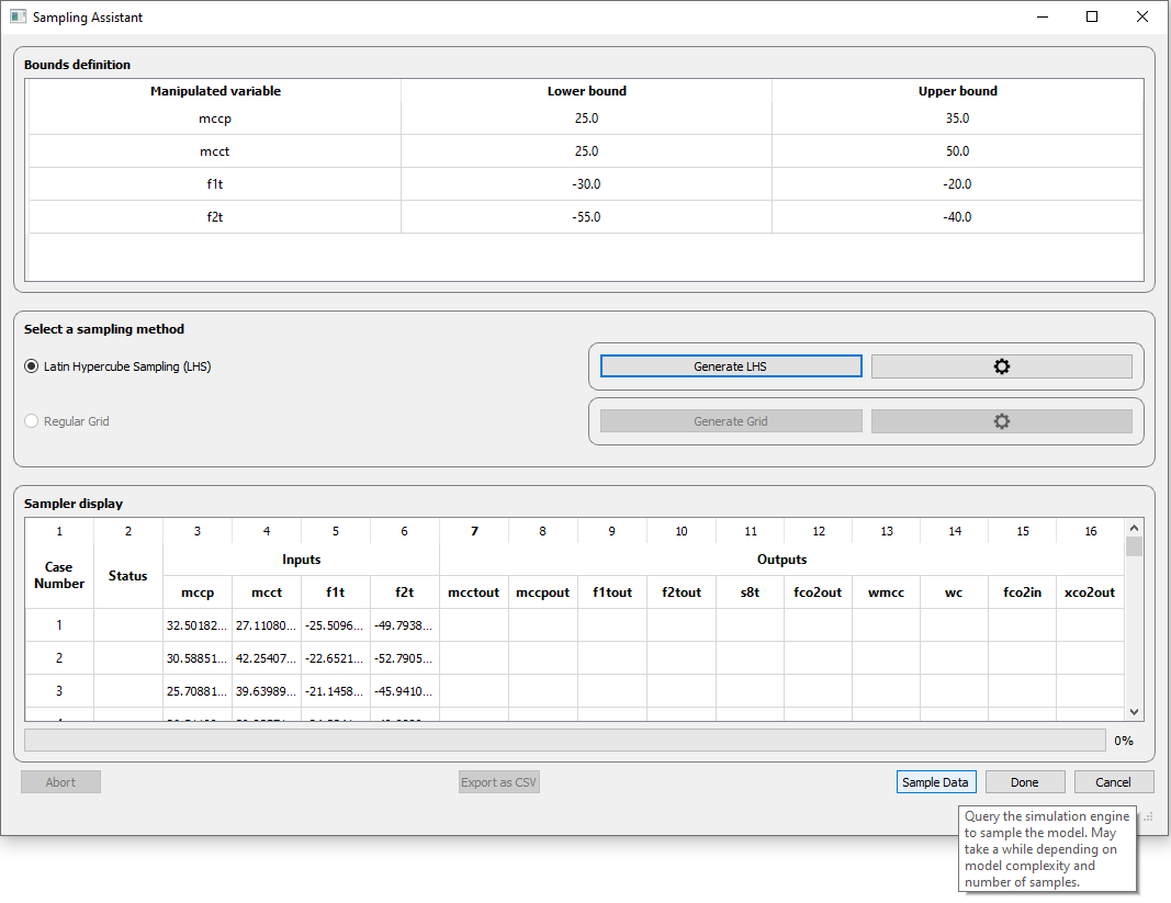
Fig. 27 Running you Design Of Experiments (DOE).

At each case, Metacontrol communicates with the Aspen Plus Engine, and collects the results automatically and in real time. You can literally see the sampling process in front of you, with the “Sampler Display” panel being updated as the cases run. Note that there is a progress bar to show you the overall process.

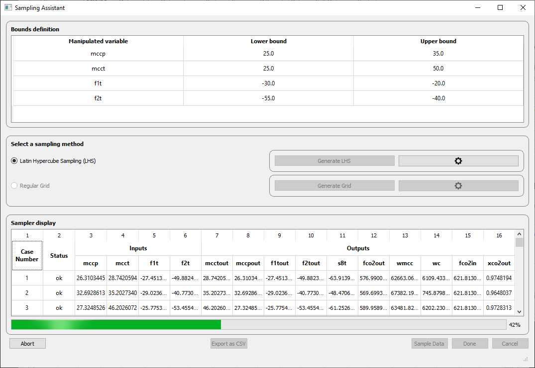
Fig. 28 Running you Design Of Experiments (DOE): Notice that you are able to abort this at any moment, simply hitting the “Abort” button at the left corner.

DOE Results panel

After the sampling process is complete, you can click on “Done”, to save your progress and your sampled data. If you click in “Cancel”, the sampling is discarded and if you click in “Export as CSV”, you will be able to save your design of experiments as a .csv file at your computer if you want.

After clicking in “Done”, you will be sent to the Sampling tab and you will notice that your data is displayed under the “DOE Results” panel. With this, you are able to go to the next tab: Metamodel.

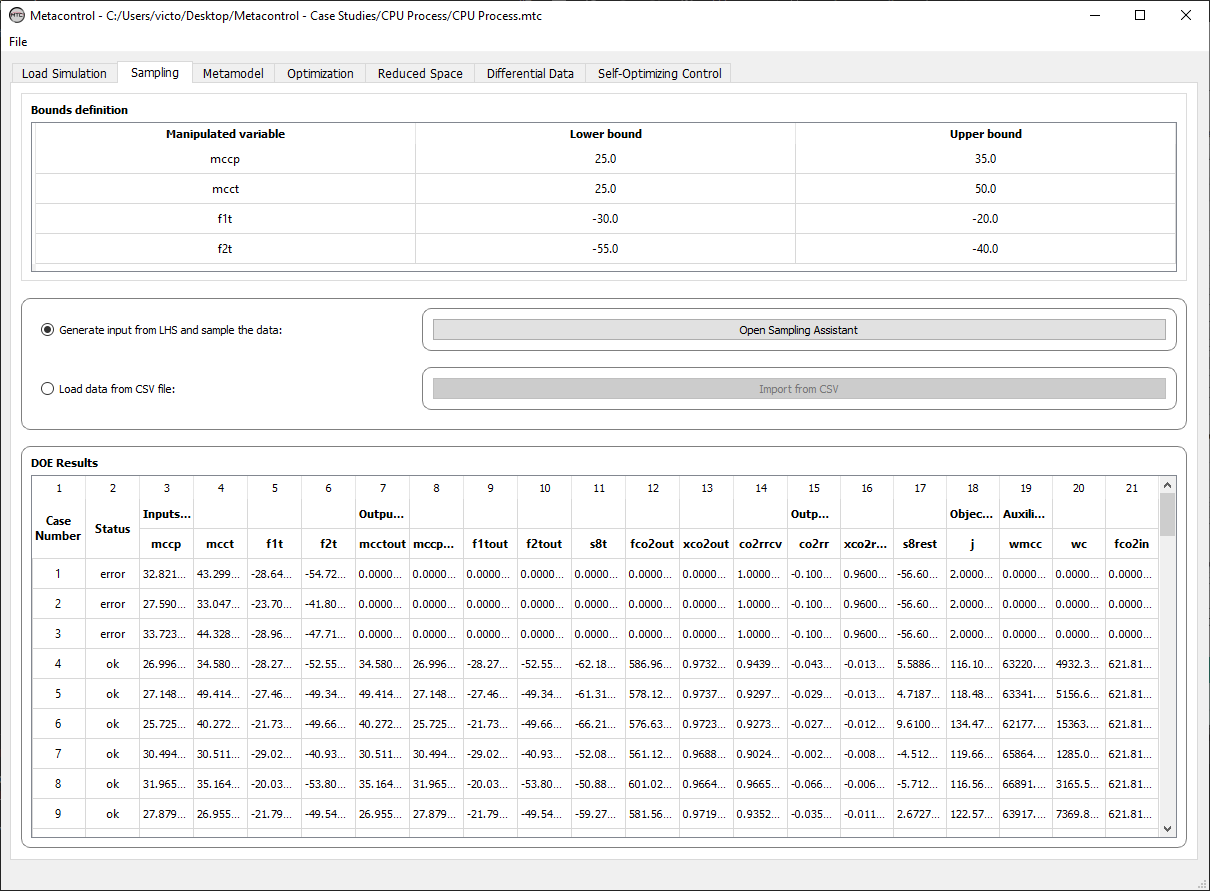
Fig. 29 Your Design Of Experiments (DOE) with all data generated, after consulting Aspen Plus.